Plot basic things with Makie

This is the Makie.jl companion to the Plot basic things guide. It shows the same examples, but built from the underlying data functions (horizontalslice, meridionalslice, zonalmean, depthprofile — re-exported from OceanGrids) and rendered with Makie plotting calls instead of AIBECS' Plots.jl recipes.

This guide is organized as follows

• Horizontal maps

• Vertical slices

• Depth profiles

• Makie extras

We use the CairoMakie backend because the docs build runs headless in CI (no display server). For interactive work, GLMakie or WGLMakie use the same plotting API.

using AIBECS
using CairoMakie
using JLD2 # required by `OCIM2.load`
using Unitful
using Unitful: ustrip
CairoMakie.activate!(type = "png")

grd, _ = OCIM2.load()
dummy = cosd.(latvec(grd))

200160-element Vector{Float64}:
 0.3221204417984906
 0.3546048870425357
 0.38666674294141884
 0.41826780077556525
 0.44937040096716135
 0.4799374779597864
 0.5099326043901359
 0.5393200344991993
 0.5680647467311559
 0.5961324854692254
 ⋮
 0.8854560256532099
 0.8688879687250066
 0.9154080085253663
 0.9009688679024191
 0.8854560256532099
 0.8688879687250066
 0.9154080085253663
 0.9009688679024191
 0.8854560256532099

A note on what's manual — AIBECS does not yet ship Makie recipes to mirror its Plots.jl ones, so every Makie plot below has to:

1. compute the slice / integral / average ahead of time via horizontalslice, meridionalslice, zonalmean, depthprofile, etc. — there is no recipe layer that calls them under the hood;

2. supply tick labels manually — Makie doesn't know that "60°N" is the nice display label for lat = 60, so we pass an explicit (positions, labels) tuple as xticks / yticks. (Once the ticks read "30°N", "60°E", …, the latitude/longitude axis labels become redundant and we drop them entirely.);

3. supply remaining axis labels manually ("Depth (m)", etc.);

4. strip Unitful values with ustrip before plotting and put the unit back on the axis or colorbar label.

That is the main trade-off vs. the Plots.jl recipes. In exchange, Makie's layout system (multiple Axis per Figure, shared colorbars, scatter compositing) comes for free — see Makie extras below.

Strip the grid axis vectors once and pre-compute the lon/lat tick vectors we'll reuse throughout. These mirror the lonticks and latticks defined inside AIBECSRecipesBaseExt:

lon = ustrip.(grd.lon)
lat = ustrip.(grd.lat)
depth = ustrip.(grd.depth)
latticks = (-90:30:90, ["90°S", "60°S", "30°S", "0°", "30°N", "60°N", "90°N"])
lonticks = (0:60:360, ["0°", "60°E", "120°E", "180°", "120°W", "60°W", "0°"])

(0:60:360, ["0°", "60°E", "120°E", "180°", "120°W", "60°W", "0°"])

Horizontal plots

Horizontal slice

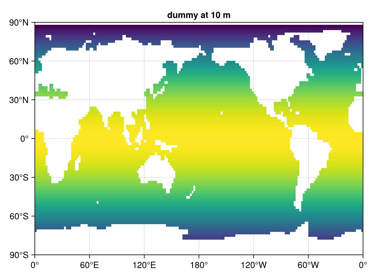
To mirror plothorizontalslice(dummy, grd, depth = 10), build the slice with horizontalslice and pass it to Makie's heatmap. Note the transpose: AIBECS' horizontalslice returns (n_lat, n_lon), while Makie's heatmap(x, y, z) expects z to have shape (length(x), length(y)).

slice = AIBECS.horizontalslice(dummy, grd; depth = 10)
heatmap(lon, lat, slice';
    axis = (
        xticks = lonticks,
        yticks = latticks,
        title = "dummy at 10 m",
    ),
)

horizontalslice accepts the same Unitful depth values as the recipe-based version:

heatmap(lon, lat, AIBECS.horizontalslice(dummy, grd; depth = 10u"m")';
    axis = (xticks = lonticks, yticks = latticks))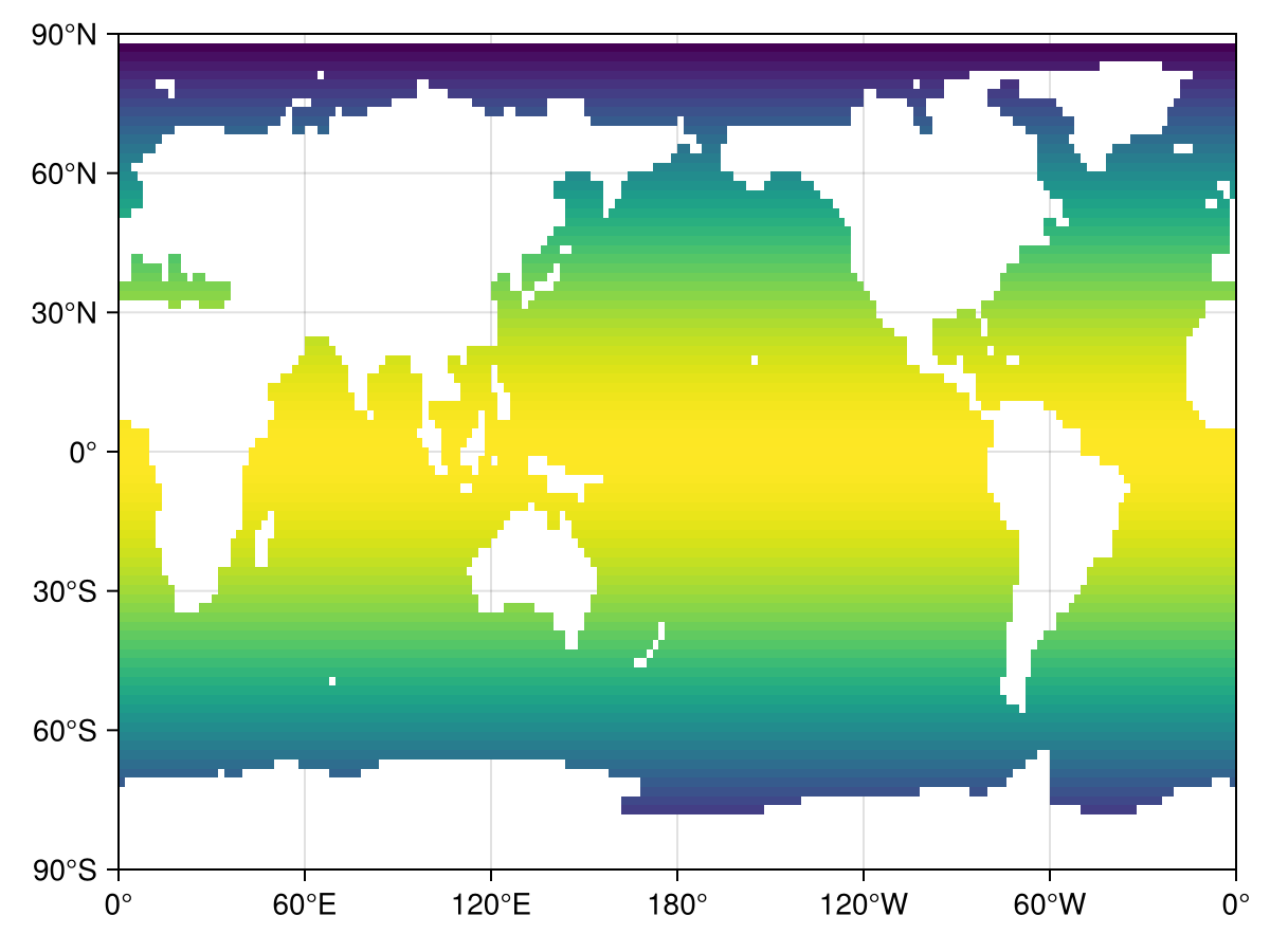

And different unit prefixes are converted under the hood by horizontalslice itself:

heatmap(lon, lat, AIBECS.horizontalslice(dummy, grd; depth = 3u"km")';
    axis = (xticks = lonticks, yticks = latticks))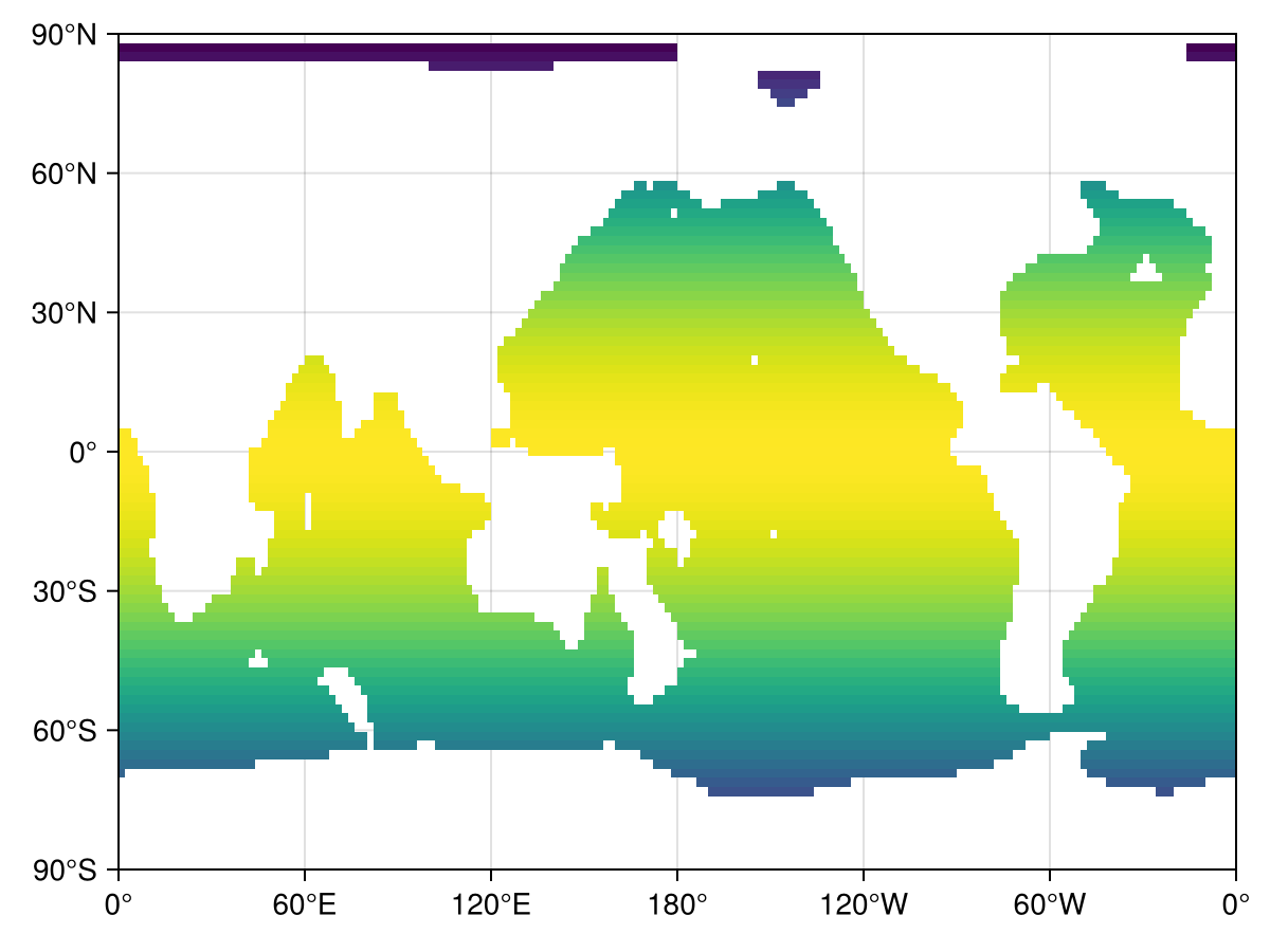

When the tracer carries units, we strip them at the call site and put the unit in the colorbar label. Makie's rich / superscript API gives typographic super/subscripts — nicer than relying on Unicode characters:

slice_units = AIBECS.horizontalslice(dummy * u"mol/m^3", grd; depth = 10u"m")
fig = Figure()
ax = Axis(fig[1, 1]; xticks = lonticks, yticks = latticks)
hm = heatmap!(ax, lon, lat, ustrip.(u"mol/m^3", slice_units)')
Colorbar(fig[1, 2], hm;
    label = rich("dummy (mol m", superscript("−3"), ")"))
fig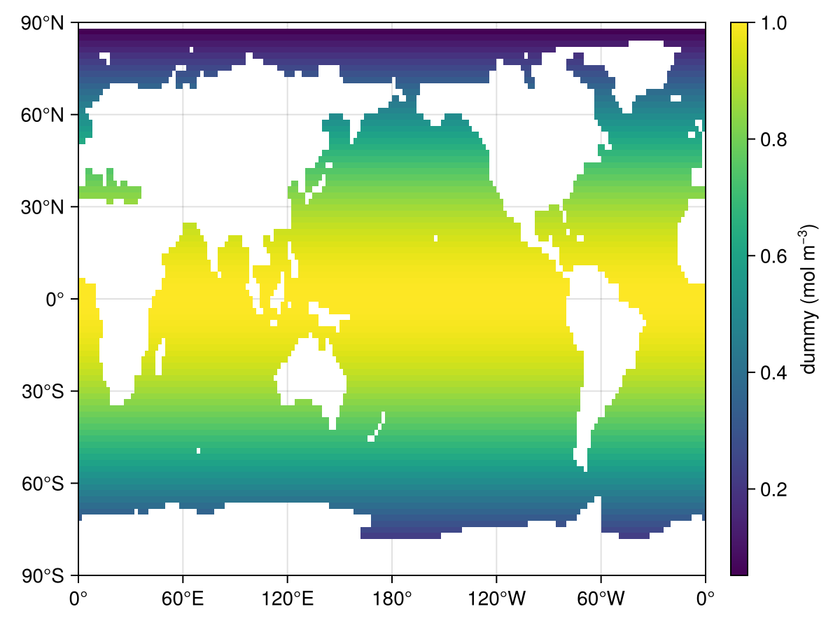

Picking a colormap is a keyword on the plot call, just like with Plots.jl. Any colormap from ColorSchemes.jl can be used. The remaining axis/colorbar fine-tuning that plot!(plt, xlabel = …, title = …, …) does in the recipe example happens inline on the Axis and Colorbar constructors:

dummy .*= cosd.(lonvec(grd))
slice_balance = AIBECS.horizontalslice(dummy, grd; depth = 100)
fig = Figure()
ax = Axis(fig[1, 1];
    xticks = lonticks, yticks = latticks,
    title = "The pacific as a whole")
hm = heatmap!(ax, lon, lat, slice_balance'; colormap = :balance)
Colorbar(fig[1, 2], hm; label = "dummy value")
fig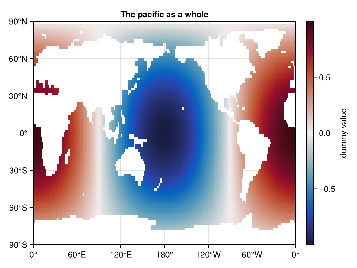

Vertical plots

Meridional slice

meridionalslice returns (n_depth, n_lat); we transpose for Makie and reverse the depth axis with yreversed = true:

dummy = cosd.(latvec(grd))
dummy .+= sqrt.(depthvec(grd)) / 30

mer = AIBECS.meridionalslice(dummy, grd; lon = 330)
heatmap(lat, depth, mer';
    axis = (
        ylabel = "Depth (m)",
        xticks = latticks,
        yreversed = true,
        title = "Meridional slice at 330° E",
    ),
)

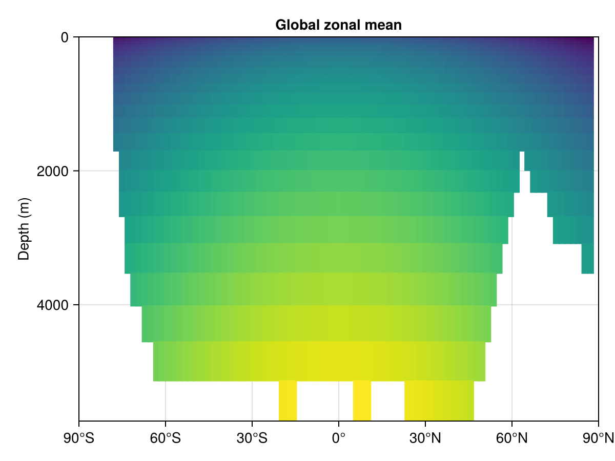
Global zonal mean

zonalmean already returns (n_lat, n_depth) (the AIBECS recipe transposes it before handing it to Plots), so no transpose is needed for Makie:

zmean = AIBECS.zonalmean(dummy, grd, 1)
heatmap(lat, depth, zmean;
    axis = (
        ylabel = "Depth (m)",
        xticks = latticks,
        yreversed = true,
        title = "Global zonal mean",
    ),
)

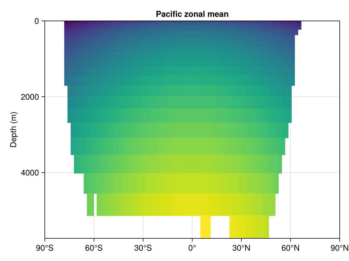
Basin-masked zonal mean

As in the Plots.jl version, basin masks come from OceanBasins.jl:

using OceanBasins
OCEANS = oceanpolygons()
mPAC = ispacific(latvec(grd), lonvec(grd), OCEANS)
zmean_PAC = AIBECS.zonalmean(dummy, grd, mPAC)
heatmap(lat, depth, zmean_PAC;
    axis = (
        ylabel = "Depth (m)",
        xticks = latticks,
        yreversed = true,
        title = "Pacific zonal mean",
    ),
)

Another meridional slice

heatmap(lat, depth, AIBECS.meridionalslice(dummy, grd; lon = -30)';
    axis = (ylabel = "Depth (m)",
            xticks = latticks,
            yreversed = true, title = "Meridional slice at -30° E"))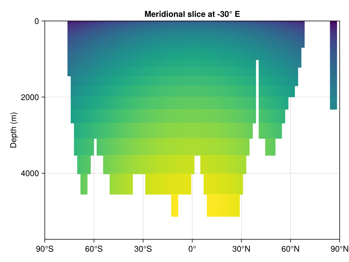

Depth profiles

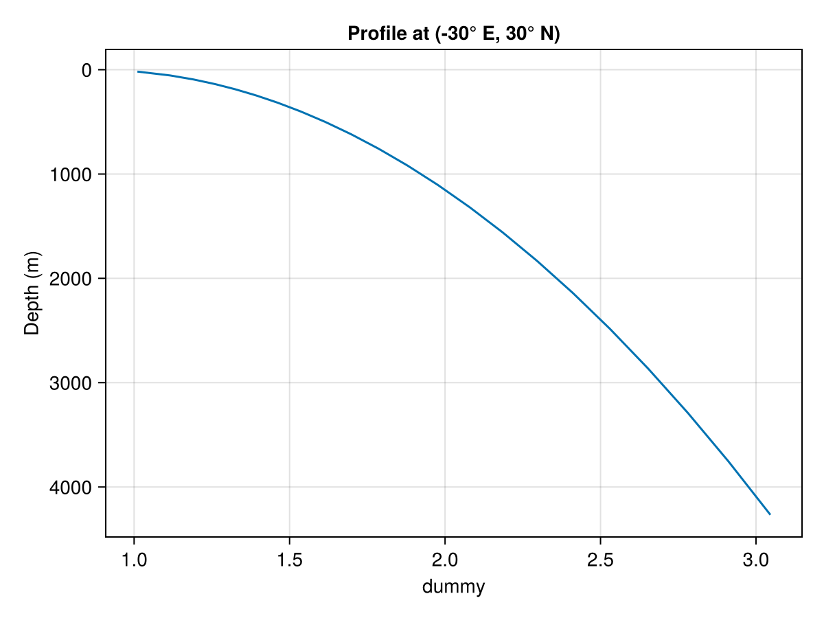
Depth profiles are 1-D — Makie's lines is the natural call. We put depth on the y-axis and flip it:

prof = AIBECS.depthprofile(dummy, grd; lonlat = (-30, 30))
lines(prof, depth;
    axis = (
        xlabel = "dummy",
        ylabel = "Depth (m)",
        yreversed = true,
        title = "Profile at (-30° E, 30° N)",
    ),
)

Makie extras

A few patterns Makie's layout system makes easy that are awkward with Plots.jl recipes.

Two horizontal slices side by side with a shared colorbar

Build a Figure, place two Axis objects in a 1×2 grid, plot into each, and share a single Colorbar:

dummy_h = cosd.(latvec(grd)) .* cosd.(lonvec(grd))
slice_surf = AIBECS.horizontalslice(dummy_h, grd; depth = 10u"m")
slice_deep = AIBECS.horizontalslice(dummy_h, grd; depth = 1000u"m")

cvals = filter(!isnan, vcat(vec(slice_surf), vec(slice_deep)))
vmin, vmax = extrema(cvals)

fig = Figure(size = (900, 350))
ax1 = Axis(fig[1, 1]; title = "10 m",
    xticks = lonticks, yticks = latticks)
ax2 = Axis(fig[1, 2]; title = "1000 m",
    xticks = lonticks, yticks = latticks)
hideydecorations!(ax2; grid = false)
hm1 = heatmap!(ax1, lon, lat, slice_surf'; colorrange = (vmin, vmax))
heatmap!(ax2, lon, lat, slice_deep'; colorrange = (vmin, vmax))
Colorbar(fig[1, 3], hm1; label = "dummy value")
fig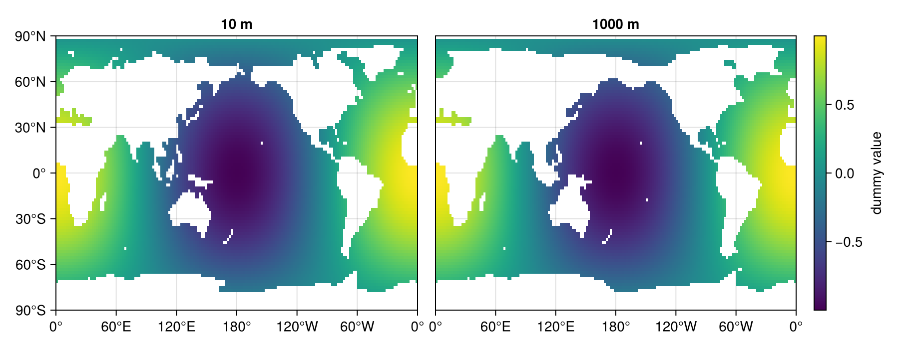

Overlay a station marker on a horizontal slice

Compositing with scatter! on the same Axis is a one-liner:

station_lon, station_lat = -30.0, 30.0
fig = Figure()
ax = Axis(fig[1, 1]; xticks = lonticks, yticks = latticks)
hm = heatmap!(ax, lon, lat, slice_surf')
scatter!(ax, [mod(station_lon, 360)], [station_lat];
    color = :red, markersize = 16, marker = :star5)
Colorbar(fig[1, 2], hm; label = "dummy value")
fig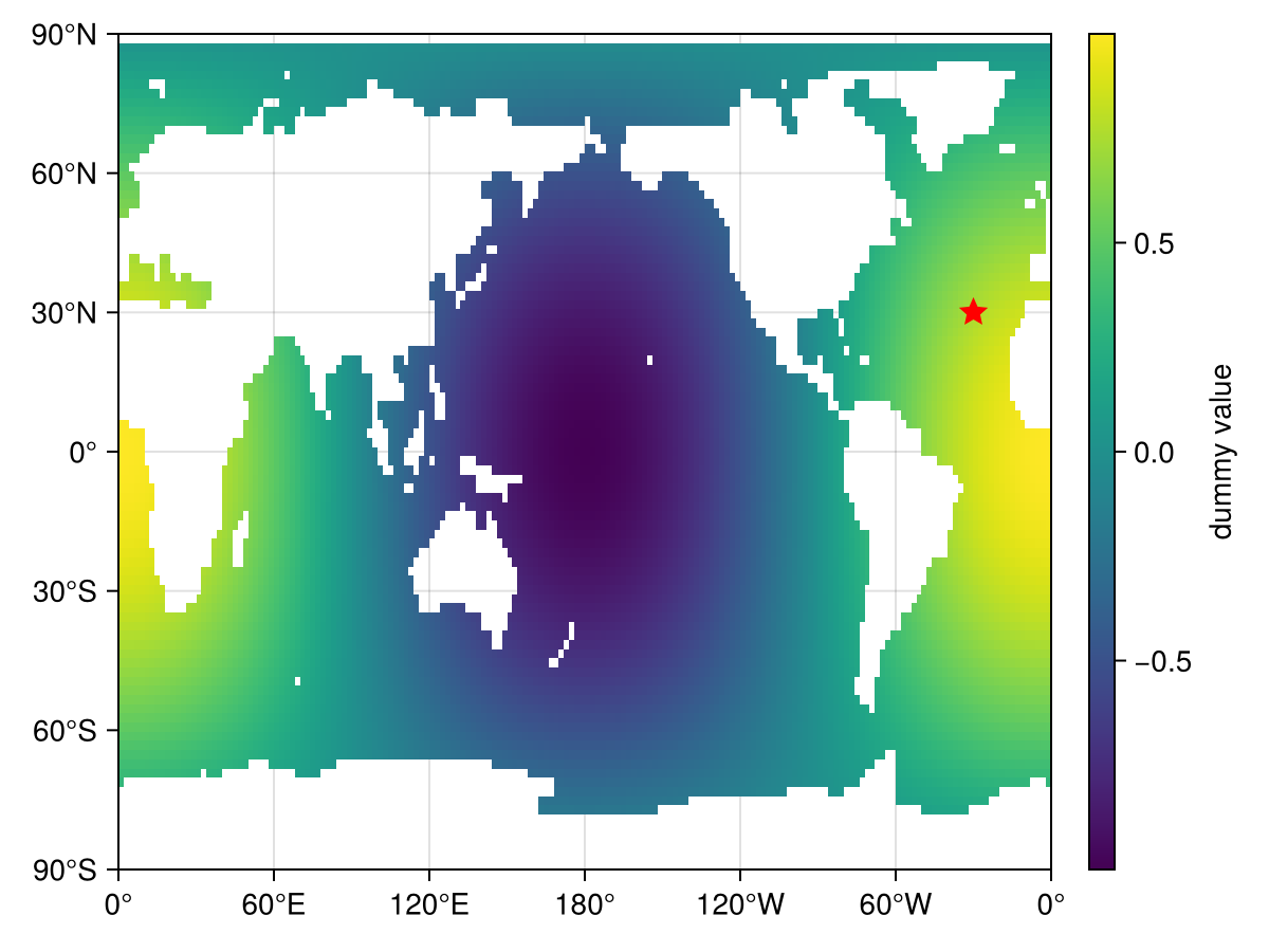

A composed multi-panel figure

A more elaborate Figure exercising many of Makie's layout primitives in one go. Patterns demonstrated:

• Three nested GridLayouts (ga, gb, gc) with different plot types in each.

• Linked axes + hidden inner decorations so shared tick / axis labels aren't repeated across columns or rows.

• Per-basin column sizing for the zonal means — each column is sized in proportion to its wet-cell latitude range, so we don't waste plot space on dry latitudes.

• Column titles via Label rather than Axis titles, so they sit in dedicated grid cells and don't fight the alphabetical corner labels.

• Resized colorbars (cb.width = Relative(...) / cb.height = Relative(...)) with flipaxis = false to put the label/ticks on the bottom (horizontal colorbar) or left (vertical colorbars).

• Diverging tick labels with explicit + / − prefixes on the balance colorbar.

• Light-grey axis background matched with nan_color = :lightgray for the contourf plots, so land cells blend in.

• contourf for the zonal means with a reversed :Zissou1Continuous colormap.

• Profile axes flipped to top-right (xaxisposition = :top, yaxisposition = :right) with bottom and left spines hidden, and x anchored at 0.

Basin masks. OCEANS was set up earlier with oceanpolygons().

mPAC2 = ispacific2(latvec(grd), lonvec(grd), OCEANS)
mATL2 = isatlantic2(latvec(grd), lonvec(grd), OCEANS)
mIND2 = isindian2(latvec(grd), lonvec(grd), OCEANS)
mSOU  = isantarctic(latvec(grd), lonvec(grd), OCEANS)
mATL  = isatlantic(latvec(grd), lonvec(grd), OCEANS)
mIND  = isindian(latvec(grd), lonvec(grd), OCEANS)
# `mPAC` was already defined for the "Basin-masked zonal mean" example

200160-element Vector{Bool}:
 0
 0
 0
 0
 0
 0
 0
 0
 0
 0
 ⋮
 0
 0
 0
 0
 0
 0
 0
 0
 0

Pre-compute everything we'll plot.

slice_pos and slice_alt are two variants of cos(lat) (the second one modulated by 1 + 0.3·sin(2·lon)), and slice_dif is their difference — diverging around 0, perfect for the managua diverging colormap.

slice_pos = AIBECS.horizontalslice(cosd.(latvec(grd)), grd; depth = 10)
slice_alt = AIBECS.horizontalslice(
    cosd.(latvec(grd)) .* (1 .+ 0.3 .* sind.(2 .* lonvec(grd))),
    grd; depth = 10,
)
slice_dif = slice_pos .- slice_alt

# 3D tracer versions paired with the three `ga` slices, so each `gb` panel
# can show "the depth profile coming from slice 1 / 2 / 3" in its basin.
# `tracer_pos` is the existing `dummy`; `tracer_alt` mirrors `slice_alt`
# with the same `sqrt(depth)/30` background; `tracer_dif` is their diff.
tracer_pos = dummy
tracer_alt = cosd.(latvec(grd)) .* (1 .+ 0.3 .* sind.(2 .* lonvec(grd))) .+
             sqrt.(depthvec(grd)) ./ 30
tracer_dif = tracer_pos .- tracer_alt

profsby(mask) = (
    AIBECS.horizontalmean(tracer_pos, grd, mask),
    AIBECS.horizontalmean(tracer_alt, grd, mask),
    AIBECS.horizontalmean(tracer_dif, grd, mask),
)
prof_PAC = profsby(mPAC2)
prof_ATL = profsby(mATL2)
prof_IND = profsby(mIND2)
prof_SOU = profsby(mSOU)

zATL = AIBECS.zonalmean(dummy, grd, mATL)
zPAC = AIBECS.zonalmean(dummy, grd, mPAC)
zIND = AIBECS.zonalmean(dummy, grd, mIND)
zlo, zhi = extrema(filter(!isnan, vcat(vec(zATL), vec(zPAC), vec(zIND))))

(0.36420743041977705, 3.451661658059956)

Wet-cell latitude range per basin (used to crop and size each column proportionally):

function wetlatrange(zm, pad = 5)
    haswet = [any(!isnan, view(zm, i, :)) for i in eachindex(lat)]
    wetidx = findall(haswet)
    isempty(wetidx) && return (-90.0, 90.0)
    return (max(-90, lat[first(wetidx)] - pad),
            min( 90, lat[last(wetidx)]  + pad))
end
xlim_ATL = wetlatrange(zATL)
xlim_PAC = wetlatrange(zPAC)
xlim_IND = wetlatrange(zIND)

(-74.23076923076923, 28.736263736263737)

+ / − tick formatter for the diverging colorbar:

plus_minus(x) = x > 0 ? "+$(round(x, digits=2))" :
                x < 0 ? "−$(round(-x, digits=2))" : "0"

plus_minus (generic function with 1 method)

Contour levels aligned on multiples of 0.2, matching reversed-Zissou:

zlevels = floor(zlo / 0.2) * 0.2 : 0.2 : ceil(zhi / 0.2) * 0.2
zissou  = cgrad(:Zissou1Continuous, length(zlevels) - 1; categorical = true)

Depth axis (used by every zonal-mean panel): 0 m at top, ticks every 1000 m.

maxdepth_round = ceil(maximum(depth) / 1000) * 1000
gcdepthticks = (0:1000:maxdepth_round, string.(Int.(0:1000:maxdepth_round)))

(0.0:1000.0:6000.0, ["0", "1000", "2000", "3000", "4000", "5000", "6000"])

Build the figure. Top row (ga + gb) takes 2/3 of the height, bottom row (gc) takes 1/3.

fig = Figure(size = (1300, 1200))
ga = fig[1, 1]   = GridLayout()
gb = fig[1, 2]   = GridLayout()
gc = fig[2, 1:2] = GridLayout()
rowsize!(fig.layout, 1, Auto(2))
rowsize!(fig.layout, 2, Auto(1))

# ga — three stacked slices. Rows 1 and 2 share a single viridis
# colorbar; row 3 is their diff with the managua diverging colormap.
shared_lo, shared_hi = extrema(filter(!isnan,
    vcat(vec(slice_pos), vec(slice_alt))))

ax_a = Axis(ga[1, 2]; backgroundcolor = :lightgray,
    xgridvisible = false, ygridvisible = false,
    xticksmirrored = true, yticksmirrored = true,
    xticks = lonticks, yticks = latticks)
hm_a = heatmap!(ax_a, lon, lat, slice_pos';
    colormap = :viridis, colorrange = (shared_lo, shared_hi))

ax_b = Axis(ga[2, 2]; backgroundcolor = :lightgray,
    xgridvisible = false, ygridvisible = false,
    xticksmirrored = true, yticksmirrored = true,
    xticks = lonticks, yticks = latticks)
heatmap!(ax_b, lon, lat, slice_alt';
    colormap = :viridis, colorrange = (shared_lo, shared_hi))

# Single colorbar spanning rows 1–2, shared between ax_a and ax_b:
cba = Colorbar(ga[1:2, 1], hm_a; flipaxis = false,
    label = "cos(lat) variants")
cba.height = Relative(0.7)

ax_c = Axis(ga[3, 2]; backgroundcolor = :lightgray,
    xgridvisible = false, ygridvisible = false,
    xticksmirrored = true, yticksmirrored = true,
    xticks = lonticks, yticks = latticks)
diff_lim = maximum(abs, filter(!isnan, slice_dif))
hm_c = heatmap!(ax_c, lon, lat, slice_dif';
    colormap = :managua, colorrange = (-diff_lim, diff_lim))
divticks = let v = round(diff_lim, digits = 2); [-v, -v/2, 0.0, v/2, v]; end
cbb = Colorbar(ga[3, 1], hm_c; flipaxis = false,
    ticks = (divticks, plus_minus.(divticks)),
    label = "row 1 − row 2")
cbb.height = Relative(0.85)

linkxaxes!(ax_a, ax_b, ax_c)
linkyaxes!(ax_a, ax_b, ax_c)
hidexdecorations!(ax_a;  ticklabels = true, label = false, ticks = false, grid = false)
hidexdecorations!(ax_b; ticklabels = true, label = false, ticks = false, grid = false)

# Annotation on ga: straight-arrow style pointing into Pacific water.
# See <https://docs.makie.org/stable/reference/plots/annotation>.
annotation!(ax_a, -100, -30, 210, 0;
    text = "cool",
    path = Ann.Paths.Arc(-0.3),
    style = Ann.Styles.LineArrow())

# gb — 2×2 basin profiles. Each panel plots the basin-mean profile of all
# three `ga` slice tracers (positive variant, alternative variant, and their
# difference). X-axis is on top, y-axis on the (default) left, bottom and
# right spines hidden; y stops at 0 m on top, like the zonal means. No
# `xticksmirrored` / `yticksmirrored` here (per request — these mirror ticks
# are only for the heatmap / contourf axes in `ga` and `gc`).
function profile_axis(grid_pos)
    ax = Axis(grid_pos;
        xgridvisible = false, ygridvisible = false,
        xaxisposition = :top,
        yreversed = true,
        bottomspinevisible = false,
        rightspinevisible = false,
        ylabel = "depth (m)",
        limits = ((0, nothing), (0, maxdepth_round)),
        xautolimitmargin = (0.0, 0.0),
        yautolimitmargin = (0.0, 0.0))
    return ax
end

function basin_label!(ax, name; align)
    pos = align == (:right, :top)    ? (1, 1) :
          align == (:right, :bottom) ? (1, 0) :
          align == (:left,  :top)    ? (0, 1) : (0, 0)
    offset = (align[1] == :right ? -5 : 5, align[2] == :top ? -5 : 5)
    text!(ax, pos...; text = name, space = :relative,
        align, offset, font = :italic, color = :black, fontsize = 13)
end

# Helper: draw all three slice-tracer profiles on one panel.
function draw_three!(ax, (p_pos, p_alt, p_dif))
    lines!(ax, p_pos, depth; color = :dodgerblue, linewidth = 2)
    lines!(ax, p_alt, depth; color = :firebrick,  linewidth = 2, linestyle = :dash)
    lines!(ax, p_dif, depth; color = :darkorange, linewidth = 2, linestyle = :dot)
end

ax_d = profile_axis(gb[1, 1]); draw_three!(ax_d, prof_PAC)
ax_e = profile_axis(gb[1, 2]); draw_three!(ax_e, prof_ATL)
ax_f = profile_axis(gb[2, 1]); draw_three!(ax_f, prof_IND)
ax_g = profile_axis(gb[2, 2]); draw_three!(ax_g, prof_SOU)

# Basin names in the top-right corner of each profile axis
basin_label!(ax_d, "Pacific";        align = (:right, :top))
basin_label!(ax_e, "Atlantic";       align = (:right, :top))
basin_label!(ax_f, "Indian";         align = (:right, :top))
basin_label!(ax_g, "Southern Ocean"; align = (:right, :top))

linkxaxes!(ax_d, ax_e, ax_f, ax_g)
linkyaxes!(ax_d, ax_e, ax_f, ax_g)
# Inner edges: hide redundant tick labels but keep the basin xlabel everywhere.
# With y-axis back on the left, the right column gets its y-decorations hidden.
hidexdecorations!(ax_f; ticklabels = true, label = false, ticks = false, grid = false)
hidexdecorations!(ax_g; ticklabels = true, label = false, ticks = false, grid = false)
hideydecorations!(ax_e; ticklabels = true, label = true,  ticks = false, grid = false)
hideydecorations!(ax_g; ticklabels = true, label = true,  ticks = false, grid = false)

# Annotation on gb: curved (Path) arrow pointing at a data point on the
# Pacific `tracer_pos` profile at depth ≈ 1500 m.
let
    idx = argmin(abs.(depth .- 1500))
    tx, ty = prof_PAC[1][idx], depth[idx]
    annotation!(ax_d, -80, -60, tx, ty;
        text = "This data point,\nright here,\nofficer",
        style = Ann.Styles.LineArrow())
end

# gc — 1×3 zonal means with `contourf`, reversed Zissou, shared horizontal cbar.
# `xticksmirrored` / `yticksmirrored` draw tick marks on all four sides of every
# panel; `yaxisposition = :right` on the rightmost panel (`ax_j`, the (j) tile)
# is what actually carries the depth tick labels and "depth (m)" axis label —
# everywhere else the y-tick labels are hidden so they're not repeated across
# columns. `yautolimitmargin = (0, 0)` plus the constructor `limits` pin the
# y-axis at exactly 0 m on top.
function zonal_axis(grid_pos, xlim; ylabel = "", yposition = :left)
    ax = Axis(grid_pos;
        backgroundcolor = :lightgray,
        xgridvisible = false, ygridvisible = false,
        xticksmirrored = true, yticksmirrored = true,
        xticks = latticks,
        yticks = gcdepthticks,
        yaxisposition = yposition,
        yreversed = true,
        limits = (xlim[1], xlim[2], 0, maxdepth_round),
        ylabel)
    return ax
end

ax_h = zonal_axis(gc[1, 1], xlim_ATL, yposition = :left, ylabel = "depth (m)")
contourf!(ax_h, lat, depth, zATL;
    levels = zlevels, colormap = zissou, nan_color = :lightgray,
    extendlow = zissou[1], extendhigh = zissou[end])

ax_i = zonal_axis(gc[1, 2], xlim_PAC)
co_i = contourf!(ax_i, lat, depth, zPAC;
    levels = zlevels, colormap = zissou, nan_color = :lightgray,
    extendlow = zissou[1], extendhigh = zissou[end])

ax_j = zonal_axis(gc[1, 3], xlim_IND)
contourf!(ax_j, lat, depth, zIND;
    levels = zlevels, colormap = zissou, nan_color = :lightgray,
    extendlow = zissou[1], extendhigh = zissou[end])

linkyaxes!(ax_h, ax_i, ax_j)
# ax_h and ax_i: keep tick *marks* via `yticksmirrored`, but hide the redundant
# tick *labels* and axis label. Only ax_j shows the depth labels (on the right).

hideydecorations!(ax_h; ticklabels = true, label = true, ticks = false, grid = false)

hideydecorations!(ax_i; ticklabels = true, label = true, ticks = false, grid = false)
hideydecorations!(ax_j; ticklabels = true, label = true, ticks = false, grid = false)

# Size each column proportional to its wet-cell latitude range:
colsize!(gc, 1, Auto(xlim_ATL[2] - xlim_ATL[1]))
colsize!(gc, 2, Auto(xlim_PAC[2] - xlim_PAC[1]))
colsize!(gc, 3, Auto(xlim_IND[2] - xlim_IND[1]))

# Basin names in the bottom-right corner of each zonal-mean panel
basin_label!(ax_h, "Atlantic"; align = (:right, :bottom))
basin_label!(ax_i, "Pacific";  align = (:right, :bottom))
basin_label!(ax_j, "Indian";   align = (:right, :bottom))

# Annotation on gc: tail-only (no arrowhead) pointing into Pacific water
# at the equator, deep ocean.
annotation!(ax_i, -100, +100, -5, 2800;
    text = "hot science",
    style = Ann.Styles.LineArrow(head = Ann.Arrows.Head()))

# Shared horizontal colorbar with label at the bottom:
cbc = Colorbar(gc[2, 1:3], co_i; vertical = false, flipaxis = false,
    label = "basin-zonal-mean dummy")
cbc.width = Relative(0.5)

# Alphabetical labels (a)–(j), bold black at the bottom-left of each axis
for (axc, lbl) in zip(
    (ax_a, ax_b, ax_c, ax_d, ax_e, ax_f, ax_g, ax_h, ax_i, ax_j),
    ("A", "B", "C", "D", "E", "F", "G", "H", "I", "J"),
)
    text!(axc, 0, 0; text = lbl, space = :relative,
        align = (:left, :bottom), offset = (5, 5),
        font = :bold, color = :black, fontsize = 19)
end

# A little breathing room between the three grid blocks:
colgap!(fig.layout, 1, 40)
rowgap!(fig.layout, 1, 40)

fig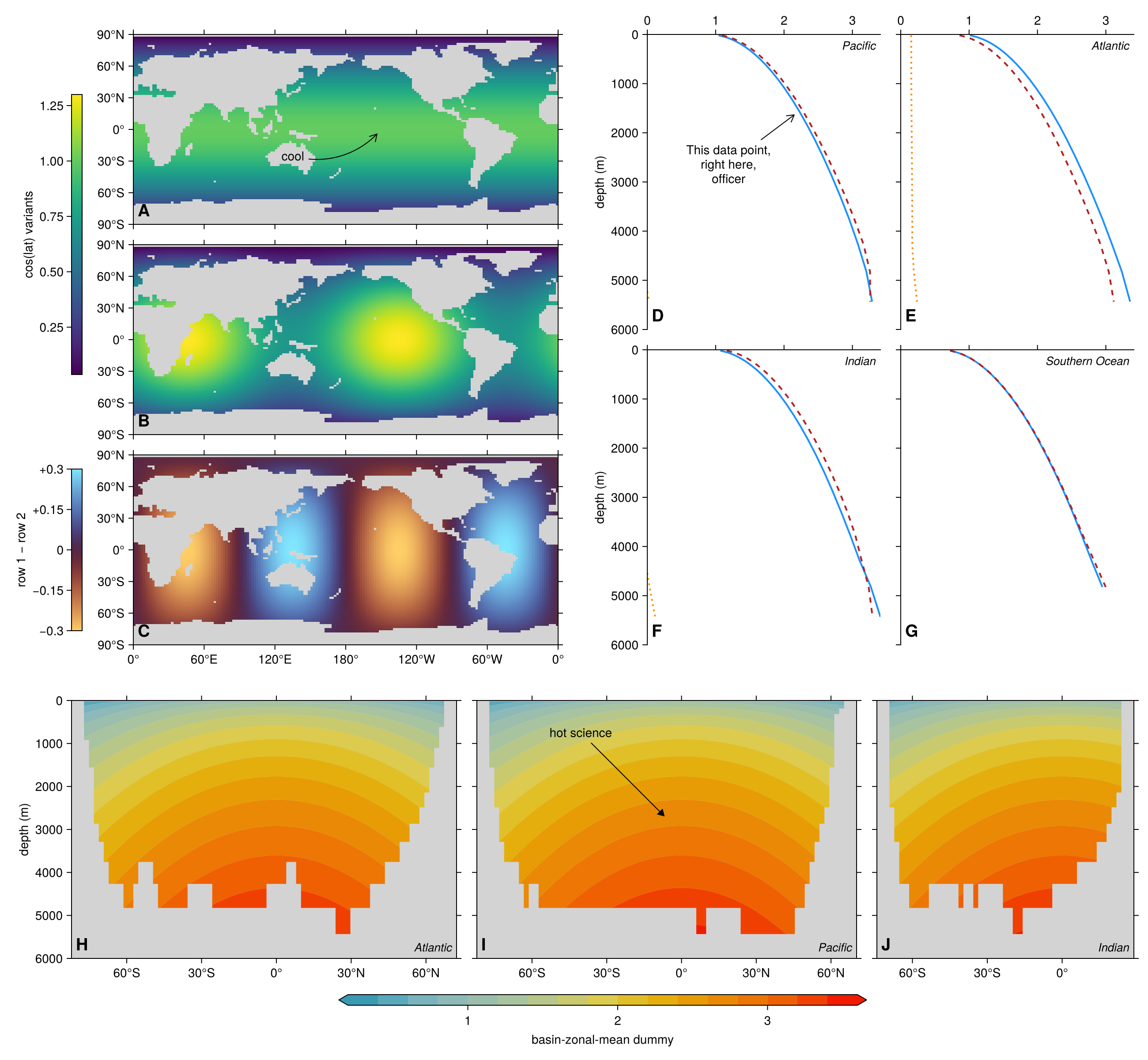

A note on geographic projections

Everything above uses the plain Cartesian Axis, so longitude / latitude are drawn as straight axes — no map projection, no coastline overlay. For real geographic plots (projections, coastlines, country borders, scale bars), see GeoMakie.jl, which adds a GeoAxis block on top of Makie. It is not used in this guide to keep the dependency footprint small and the examples focused on AIBECS' data functions, but a how-to that demonstrates GeoAxis with AIBECS output would be a welcome contribution — pull requests appreciated.

---

This page was generated using Literate.jl.