Estimate fluxes
This will take you through the process of extracting flux information from a given transport operator. It is split into 3 parts
Let's start telling Julia we will be using AIBECS and Plots.
using AIBECS
using Plots
using JLD2 # required by `OCCA.load` / `Circulation.load`
1. Operator stencil
Let's load the OCCA grid information grd and transport matrix T here).
grd, T = OCCA.load()(, sparse([1, 2, 9551, 9606, 1, 2, 3, 57, 9552, 9607 … 79928, 84632, 84659, 84660, 84661, 79891, 79929, 84633, 84660, 84661], [1, 1, 1, 1, 2, 2, 2, 2, 2, 2 … 84660, 84660, 84660, 84660, 84660, 84661, 84661, 84661, 84661, 84661], [2.2826279842870655e-7, 1.8030621712982388e-10, -2.202759122121374e-7, -1.669794081839543e-8, -8.32821319857397e-8, 3.6454996849707203e-7, -2.4345873581518986e-8, 2.346272528650749e-8, -3.294980961099172e-7, 6.798120022902578e-9 … -2.337773104642457e-8, -1.0853897038905248e-8, -2.4801404742669764e-8, 7.658935255067088e-8, -2.49410804832536e-8, -2.2788300189327118e-9, -3.386139290468414e-8, -2.0539768803799346e-8, -1.8193948479846445e-8, 5.864674518359535e-8], 84661, 84661))Multiplying
AIBECS provides a function, stencil, that returns all the relative cartesian indices (AKA the relative sub-indices) of the neighbors used by a given operator. In the case of OCCA, the stencil is thus
st = stencil(T, grd)7-element Vector{CartesianIndex{3}}:
CartesianIndex(0, 0, 0)
CartesianIndex(-1, 0, 0)
CartesianIndex(0, 1, 0)
CartesianIndex(0, 0, -1)
CartesianIndex(1, 0, 0)
CartesianIndex(0, -1, 0)
CartesianIndex(0, 0, 1)There is also a label function to, well, label the stencil elements in a more human-readable way. (Note label is not exported, so you must specify that it comes from the AIBECS package, as below.)
[st AIBECS.label.(st)]7×2 Matrix{Any}:
CartesianIndex(0, 0, 0) ""
CartesianIndex(-1, 0, 0) "South"
CartesianIndex(0, 1, 0) "East"
CartesianIndex(0, 0, -1) "Above"
CartesianIndex(1, 0, 0) "North"
CartesianIndex(0, -1, 0) "West"
CartesianIndex(0, 0, 1) "Below"The stencil can be visualized with the plotstencil recipe
plotstencil(st)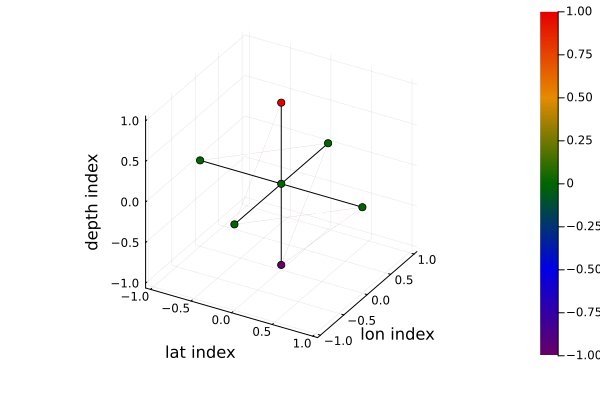
Note
The continuous equivalent of the matrix
This works for any circulation, so you can swap grd and T and try again... Here we plot the same figure for a few different circulations available in AIBECS.
plts = Any[]
for Circulation in [OCIM0, OCIM1, OCIM2, OCCA]
    grd, T = Circulation.load()
    push!(plts, plotstencil(stencil(grd, T), title = string(Circulation)))
end
plot(plts..., layout = (2, 2))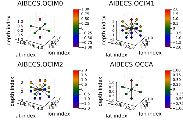
These stencils are useful to clarify the origin and destination of tracer fluxes we are going to explore in this guide..
2. Operator Partition
For a given operator
Let's take the "West" neighbor of the OCCA stencil
dir = st[findfirst(AIBECS.label.(st) .== "West")]CartesianIndex(0, -1, 0)The AIBECS provides a function directional_T that returns the transport operator corresponding to the direction provided from the stencil element.
T_West = directional_transport(T, grd, dir)84661×84661 SparseMatrixCSC{Float64, Int64} with 161878 stored entries:
⎡⠳⣄⠀⠀⠈⠀⠀⠀⠀⠀⠀⠀⠀⠀⠀⠀⠀⠀⠀⠀⠀⠀⠀⠀⠀⠀⠀⠀⠀⠀⠀⠀⠀⠀⠀⠀⠀⠀⠀⠀⎤
⎢⠀⠈⠳⣄⠀⠀⠀⠀⠀⠀⠀⠀⠀⠀⠀⠀⠀⠀⠀⠀⠀⠀⠀⠀⠀⠀⠀⠀⠀⠀⠀⠀⠀⠀⠀⠀⠀⠀⠀⠀⎥
⎢⠀⠀⠀⠈⠳⣄⠀⠀⠀⠂⠀⠀⠀⠀⠀⠀⠀⠀⠀⠀⠀⠀⠀⠀⠀⠀⠀⠀⠀⠀⠀⠀⠀⠀⠀⠀⠀⠀⠀⠀⎥
⎢⠀⠀⠀⠀⠀⠈⠳⣄⠀⠀⠀⠀⠀⠀⠀⠀⠀⠀⠀⠀⠀⠀⠀⠀⠀⠀⠀⠀⠀⠀⠀⠀⠀⠀⠀⠀⠀⠀⠀⠀⎥
⎢⠀⠀⠀⠀⠀⠀⠀⠈⠳⣄⠀⠀⠀⠄⠀⠀⠀⠀⠀⠀⠀⠀⠀⠀⠀⠀⠀⠀⠀⠀⠀⠀⠀⠀⠀⠀⠀⠀⠀⠀⎥
⎢⠀⠀⠀⠀⠀⠀⠀⠀⠀⠈⠳⣄⠀⠀⠀⠀⠀⠀⠀⠀⠀⠀⠀⠀⠀⠀⠀⠀⠀⠀⠀⠀⠀⠀⠀⠀⠀⠀⠀⠀⎥
⎢⠀⠀⠀⠀⠀⠀⠀⠀⠀⠀⠀⠈⠳⣄⠀⠀⠀⢠⠀⠀⠀⠀⠀⠀⠀⠀⠀⠀⠀⠀⠀⠀⠀⠀⠀⠀⠀⠀⠀⠀⎥
⎢⠀⠀⠀⠀⠀⠀⠀⠀⠀⠀⠀⠀⠀⠈⠳⣄⠀⠀⠀⠀⠀⠀⠀⠀⠀⠀⠀⠀⠀⠀⠀⠀⠀⠀⠀⠀⠀⠀⠀⠀⎥
⎢⠀⠀⠀⠀⠀⠀⠀⠀⠀⠀⠀⠀⠀⠀⠀⠈⠳⣄⠀⠀⠀⢀⠀⠀⠀⠀⠀⠀⠀⠀⠀⠀⠀⠀⠀⠀⠀⠀⠀⠀⎥
⎢⠀⠀⠀⠀⠀⠀⠀⠀⠀⠀⠀⠀⠀⠀⠀⠀⠀⠈⠳⣄⠀⠀⠀⠀⠀⠀⠀⠀⠀⠀⠀⠀⠀⠀⠀⠀⠀⠀⠀⠀⎥
⎢⠀⠀⠀⠀⠀⠀⠀⠀⠀⠀⠀⠀⠀⠀⠀⠀⠀⠀⠀⠈⠳⣄⠀⠀⠀⢀⠀⠀⠀⠀⠀⠀⠀⠀⠀⠀⠀⠀⠀⠀⎥
⎢⠀⠀⠀⠀⠀⠀⠀⠀⠀⠀⠀⠀⠀⠀⠀⠀⠀⠀⠀⠀⠀⠈⠳⣄⠀⠀⠀⠀⠀⠀⠀⠀⠀⠀⠀⠀⠀⠀⠀⠀⎥
⎢⠀⠀⠀⠀⠀⠀⠀⠀⠀⠀⠀⠀⠀⠀⠀⠀⠀⠀⠀⠀⠀⠀⠀⠈⠳⣄⠀⠀⠀⢀⠀⠀⠀⠀⠀⠀⠀⠀⠀⠀⎥
⎢⠀⠀⠀⠀⠀⠀⠀⠀⠀⠀⠀⠀⠀⠀⠀⠀⠀⠀⠀⠀⠀⠀⠀⠀⠀⠈⠳⣄⠀⠈⠀⠀⠀⠀⠀⠀⠀⠀⠀⠀⎥
⎢⠀⠀⠀⠀⠀⠀⠀⠀⠀⠀⠀⠀⠀⠀⠀⠀⠀⠀⠀⠀⠀⠀⠀⠀⠀⠀⠀⠈⠳⣄⠀⠀⠀⢀⠀⠀⠀⠀⠀⠀⎥
⎢⠀⠀⠀⠀⠀⠀⠀⠀⠀⠀⠀⠀⠀⠀⠀⠀⠀⠀⠀⠀⠀⠀⠀⠀⠀⠀⠀⠀⠀⠈⠳⣄⠀⠀⠀⠀⠀⠀⠀⠀⎥
⎢⠀⠀⠀⠀⠀⠀⠀⠀⠀⠀⠀⠀⠀⠀⠀⠀⠀⠀⠀⠀⠀⠀⠀⠀⠀⠀⠀⠀⠀⠀⠀⠈⠳⣄⠀⠀⠀⢀⠀⠀⎥
⎢⠀⠀⠀⠀⠀⠀⠀⠀⠀⠀⠀⠀⠀⠀⠀⠀⠀⠀⠀⠀⠀⠀⠀⠀⠀⠀⠀⠀⠀⠀⠀⠀⠀⠈⠳⣄⠀⠀⠀⠀⎥
⎢⠀⠀⠀⠀⠀⠀⠀⠀⠀⠀⠀⠀⠀⠀⠀⠀⠀⠀⠀⠀⠀⠀⠀⠀⠀⠀⠀⠀⠀⠀⠀⠀⠀⠀⠀⠈⠳⣄⠀⢀⎥
⎣⠀⠀⠀⠀⠀⠀⠀⠀⠀⠀⠀⠀⠀⠀⠀⠀⠀⠀⠀⠀⠀⠀⠀⠀⠀⠀⠀⠀⠀⠀⠀⠀⠀⠀⠀⠀⠀⠈⠳⣄⎦Notice how T_West only has nonzeros on the main diagonal and on one off-diagonal, that connect each box index with the index of the box "West" of it.
3. Flux Estimate
We can look at the depth-integrated mean flux of a fictitious tracer
nwet = count(iswet(grd))
x = ones(nwet)
plotverticalintegral(-T_West * x * u"mol/m^3/s" .|> u"μmol/m^3/s", grd, mask = depthvec(grd) .< 100, color = :seaborn_icefire_gradient, clim = 1.0e2 .* (-1, 1))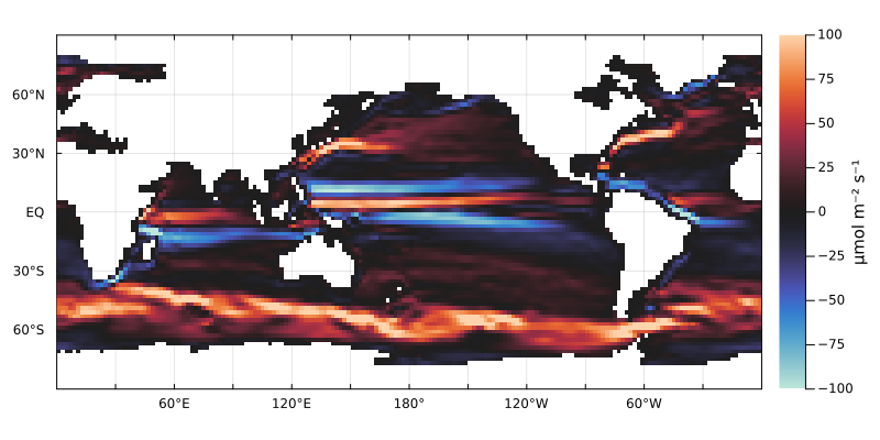
To get all the matrices for all directions you can use
directional_transports(T, grd)Dict{String, SparseMatrixCSC{Float64, Int64}} with 6 entries:
"Below" => sparse([1, 2, 3, 4, 5, 6, 7, 8, 9, 10 … 79882, 79883, 79884, 798…
"East" => sparse([9551, 2, 9552, 3, 9553, 4, 9554, 5, 9555, 6 … 84629, 846…
"Above" => sparse([9606, 9607, 9608, 9609, 9610, 9611, 9612, 9613, 9614, 9615…
"West" => sparse([1, 2, 57, 3, 58, 4, 59, 5, 60, 6 … 79925, 84657, 79926, …
"North" => sparse([1, 1, 2, 2, 3, 3, 4, 4, 5, 5 … 84656, 84656, 84657, 8465…
"South" => sparse([2, 2, 3, 3, 4, 4, 5, 5, 6, 6 … 84657, 84657, 84658, 8465…See also: the Sinking particles how-to for building flux operators from a settling-velocity profile rather than decomposing an existing circulation.
This page was generated using Literate.jl.