Plot basic things

This guide is organized as follows

Horizontal maps
Vertical slices
Depth profiles

In this guide we will focus on how-to plot things using AIBECS' built-in recipes for Plots.jl. These recipes are implemented using RecipesBase.jl, which are explained in Plots.jl's documentation.

Throughout we will use the OCIM2 grid and we will create a dummy tracer as a function of location to showcase each plot, just for the sake of the examples herein.

using Plots
using AIBECS
grd, _ = OCIM2.load()
dummy = cosd.(latvec(grd))

The most common thing you plot after a simulation of marine tracers is a horizontal slice. In this case, you just need to provide the tracer (dummy here), the grid object grd, and the depth at which you want to plot.

plothorizontalslice(dummy, grd, depth=10)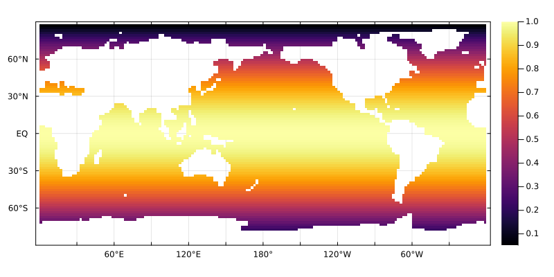

You can supply units for the depth at which you want to see the horizontal slice.

plothorizontalslice(dummy, grd, depth=10u"m")

And the units should be understood under the hood.

plothorizontalslice(dummy, grd, depth=3u"km")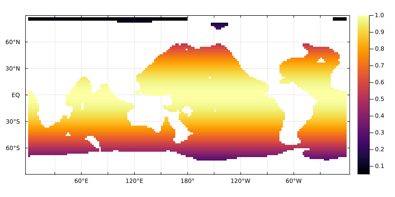

If your tracer is supplied with units, those will show in the colorbar label

plothorizontalslice(dummy * u"mol/m^3", grd, depth=10u"m")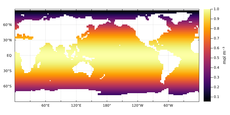

The advantage of Plots.jl recipes like this one is that you can specify other pieces of the plot as you would with built-in functions. The advantage of Plots.jl recipes like this one is that you can specify other pieces of the plot as you would with built-in functions. For example, you can chose the colormap with the color keyword argument.

dummy .*= cosd.(lonvec(grd))
plt = plothorizontalslice(dummy, grd, depth=100, color=:balance)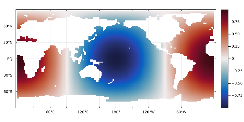

And you can finetune attributes after the plot is created.

plot!(plt, xlabel="Lon", ylabel="Lat", colorbar_title="dummy value", title="The pacific as a whole")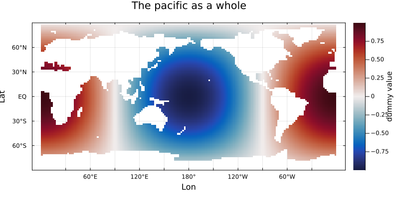

Vertical plots

Exploring the vertical distribution of tracers is important after all.

Zonal slices

You must specify the longitude

dummy = cosd.(latvec(grd))
dummy .+= sqrt.(depthvec(grd)) / 30
plotmeridionalslice(dummy, grd, lon=330)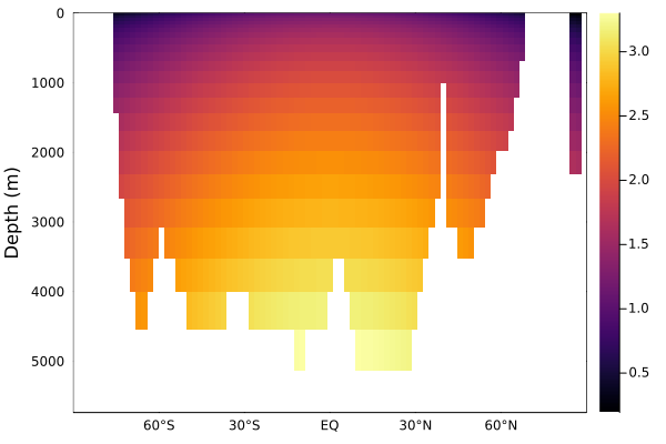

Zonal averages

Global zonal average

zonalaverage(dummy, grd)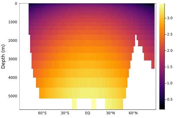

If you want a zonal average over a specific region, you can just mask it out

Basin zonal average

This is experimental at this stage and relies on OceanBasins.jl. You can create basin masks using this package with

using OceanBasins
OCEANS = oceanpolygons()
basins = sum(i*isbasin(latvec(grd), lonvec(grd), OCEANS) for (i,isbasin) in enumerate([isindian2, ispacific2, isatlantic2, isantarctic]))
plothorizontalslice(basins, grd, depth=0, seriestype=:heatmap, color=:lightrainbow)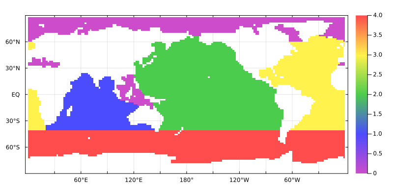

and you can mask a specific region with the mask keyword argument

mPAC = ispacific(latvec(grd), lonvec(grd), OCEANS)
plotzonalaverage(dummy, grd, mask=mPAC)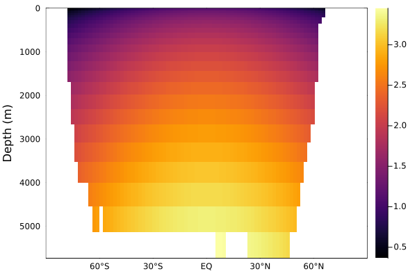

Meridional slices

Just as you should expect at this stage, you can plot a meridional slice with

plotmeridionalslice(dummy, grd, lon=-30)

Depth profiles

Sometimes you want a profile at a given station or location

plotdepthprofile(dummy, grd, lonlat=(-30,30))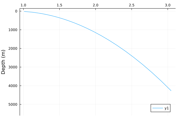

This page was generated using Literate.jl.