Steady-state solvers

Finding a steady state of   runs an outer nonlinear solver that calls an inner linear solver at every Jacobian-update / Newton-step iteration. AIBECS lets you pick each component independently:

• The outer nonlinear solver can be any algorithm from NonlinearSolve.jl (NewtonRaphson, TrustRegion, LimitedMemoryBroyden, …), or AIBECS's own CTKAlg — a bespoke Newton–Chord–Shamanskii method adapted from C. T. Kelley's MATLAB implementations (Kelley, 2003) and specialised to the AIBECS state Jacobian.

• The inner linear solver can be any factorisation from LinearSolve.jl — usually a sparse direct factorisation (UMFPACKFactorization, KLUFactorization, MKLPardisoFactorize).

The NonlinearSolve how-to walks through the call pattern for the SciML side. For CTKAlg the call is just solve(prob, CTKAlg()).

Recommended pairing: CTKAlg() + UMFPACKFactorization()

Calling CTKAlg() with no arguments yields CTKAlg(linsolve = UMFPACKFactorization()) — the AIBECS-recommended default. Two reasons it's the recommendation:

1. CTKAlg uses a Shamanskii update. The Newton iteration only refreshes the Jacobian when the residual stops shrinking fast enough (r > rSham₀ = 0.5). On AIBECS systems where the steady-state Jacobian changes slowly between iterations, one factorisation typically covers several Newton steps — generally faster in our experience than the "refresh every iteration" baseline that NewtonRaphson uses. The tradeoff is robustness: when the Jacobian does drift, Shamanskii's stale factors can take an extra Newton step to recover. Armijo line search is the safety net.

2. UMFPACKFactorization reuses its factors. CTKAlg runs the linear solve through a LinearSolve.LinearCache, so when Shamanskii recycles the Jacobian, UMFPACK's LU factors are reused directly — no refactorisation. Pairing CTKAlg with a factorisation that supports cache reuse is what makes the Shamanskii win compound.

If CTKAlg fails to converge on a pathological problem, the standard fallback is NewtonRaphson (still with UMFPACK) via the NonlinearSolve route below — fresh Jacobian every iteration, slower but more forgiving. More robust schemes still — for example pseudo-transient continuation (NonlinearSolve.PseudoTransient), which embeds the steady-state problem in a fictitious time evolution and is known to help on stiff systems — may also be worth trying; we have not benchmarked them on AIBECS systems.

When to use the NonlinearSolve route instead

• You want a different outer algorithm (TrustRegion, LimitedMemoryBroyden, …).

• You want to benchmark several algorithms against CTKAlg on your own circulation.

• You need NonlinearSolve features that CTKAlg does not surface (custom termination modes, callbacks, sensitivity hooks).

The cost is the load-time of NonlinearSolve.jl and LinearSolve.jl plus their transitive deps — neither is a hard AIBECS dependency. The underlying SteadyStateProblem and sparse Jacobian are reused across both routes; switching is a one-line change at the call site.

Verified algorithm/factorisation pairs

The combinations below have been checked on the toy Primeau_2x2x2 circulation and converge to the same root as CTKAlg().

Solver call	Match vs CTKAlg()	Notes
solve(prob, CTKAlg())	(baseline)	Native AIBECS Newton–Chord–Shamanskii; CTKAlg + UMFPACK default.
solve(nlprob, NewtonRaphson(linsolve = UMFPACKFactorization()))	exact	Recommended NonlinearSolve fallback.
solve(nlprob, NewtonRaphson(linsolve = KLUFactorization()))	1e-10	KLU may win on very-sparse Jacobians.
solve(nlprob, AIBECS.recommended_nlalg())	exact	Convenience for NewtonRaphson + UMFPACK.

For the NonlinearSolve rows, nlprob = AIBECS.nonlinearproblem(prob) — see the how-to for the full pattern. The helper attaches the sparse Jacobian buffer type so LinearSolve's UMFPACK / KLU factorisations allocate sparse buffers instead of erroring on a dense default.

Stopping rule used in the benchmark

To keep the comparison apples-to-apples, every solver below is invoked with the same termination configuration, exposed as a helper:

solve(prob, alg; AIBECS.default_termination_condition()...)

default_termination_condition() returns the (termination_condition, abstol, reltol) triple CTKAlg uses by default — NormTerminationMode on the residual ∞-norm with reltol = 1 / (1 Myr in seconds) ≈ 3.17e-14 and abstol = 0. The criterion reads physically as "the system's typical change timescale exceeds 1 Myr." NonlinearSolve algorithms (NewtonRaphson, TrustRegion, …) accept this configuration directly.

Small benchmark showcase

The numbers below come from benchmark/solvers.jl, regenerated on every docs CI build. This is not a solver-selection guide. Steady-state solver performance is highly problem-specific, and the suite below only covers a small set of AIBECS-shaped problems on single-tracer (idealage, radiocarbon) and two-tracer (po4pop) setups with OCCA and OCIM0. Use these as evidence that CTKAlg() + UMFPACKFactorization() tends to win in the cases benchmarked here — not as a prescription for arbitrary tracer setups.

The harness runs two orthogonal sweeps, both anchored at the AIBECS recommendation CTKAlg + UMFPACK:

1. Linear-solver sweep — CTKAlg is held fixed as the nonlinear engine, and the inner linsolve is varied (UMFPACK, KLU, Sparspak, and MKL Pardiso on Linux CI).

2. Nonlinear-solver sweep — UMFPACK is held fixed as the linear solver, and the outer nonlinear algorithm is varied (CTKAlg, NewtonRaphson).

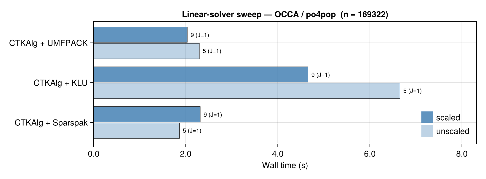
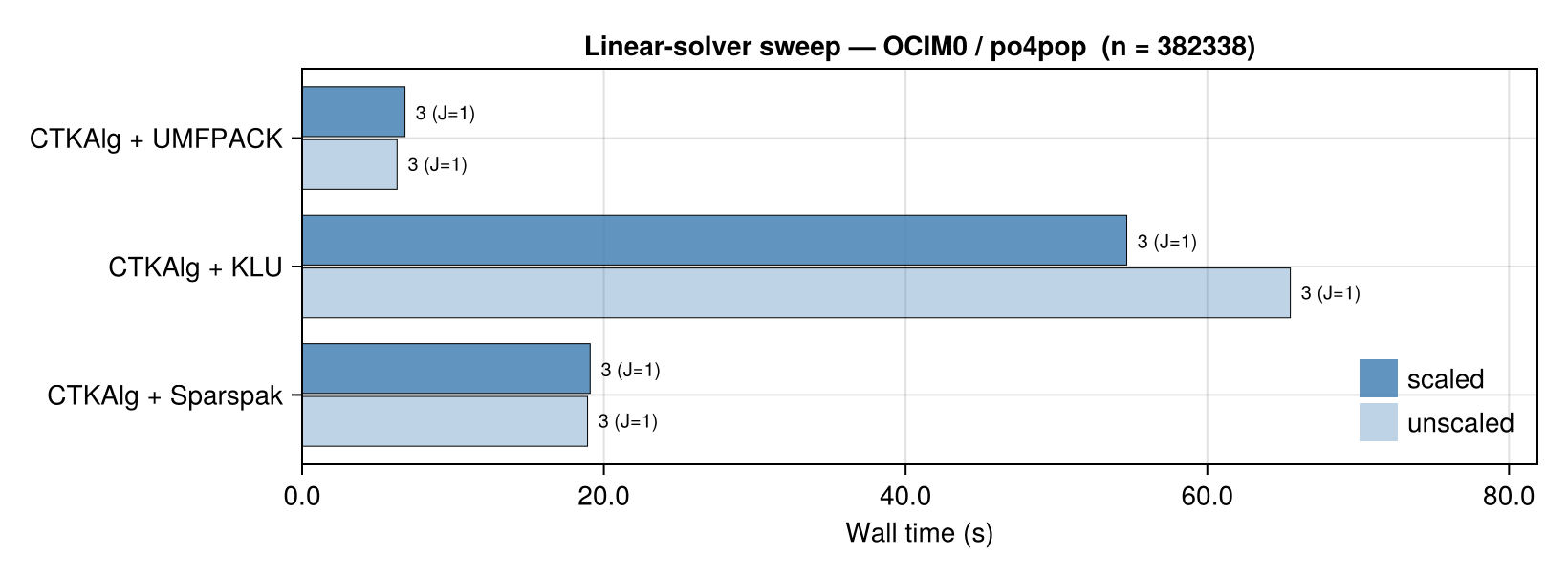
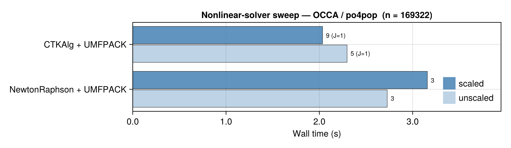
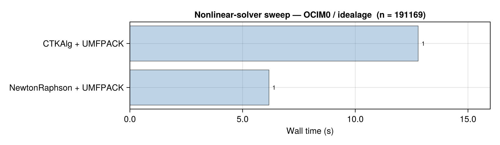
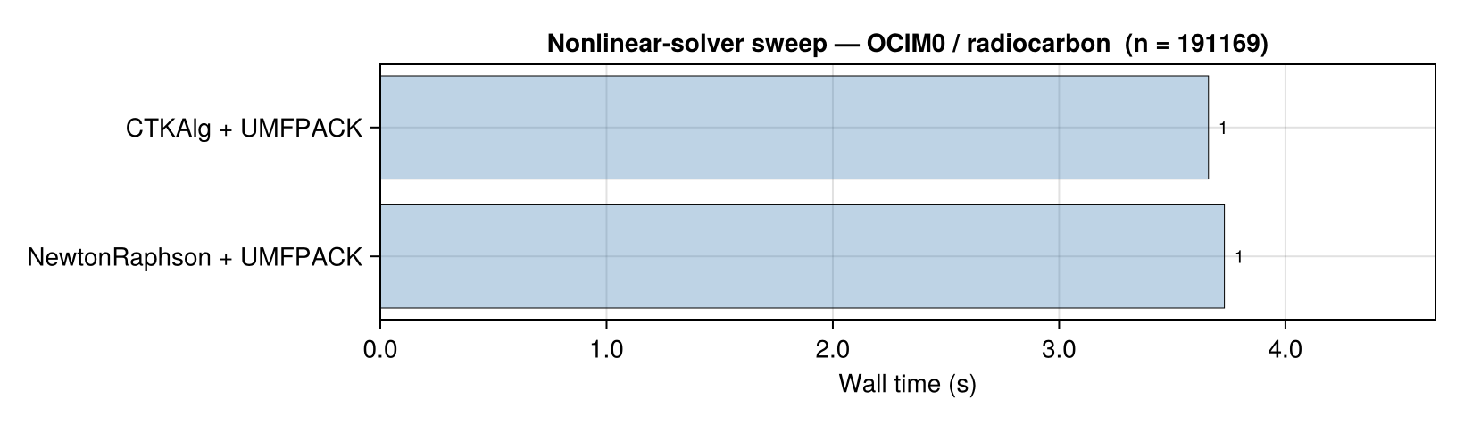
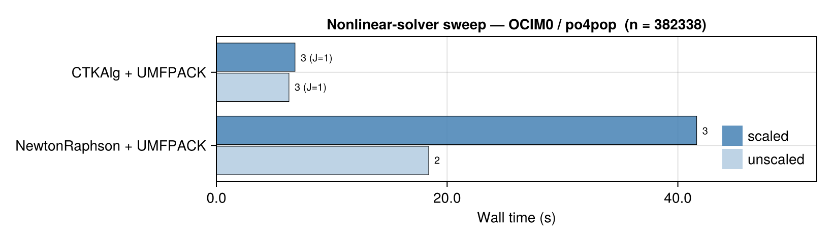
Each figure below is a horizontal-bar panel for one (circulation, tracer) cell, with text annotations to the right of each bar showing Newton iterations (and Jacobian-refresh count when it differs — a sign of CTKAlg's Shamanskii recycling). Where the setup ships physics-based scales (po4pop), each algorithm gets two bars per row — filled (scaled, nondimensionalize applied) and open (unscaled). Single-tracer setups (idealage, radiocarbon) lack a meaningful scaling and show only one bar per algorithm row. Rows whose solver returned a non-success retcode are omitted from the figure (the table below still records them in the Retcode column).

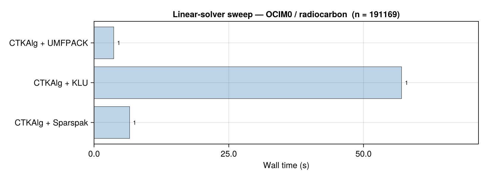
Linear-solver sweep

CTKAlg held fixed; linsolve varied. KLU, Sparspak, and MKL Pardiso are exercised here (and only here) — pairing slow linear solvers with multiple nonlinear wrappers would dominate run wall time without adding signal.

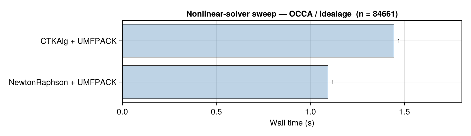
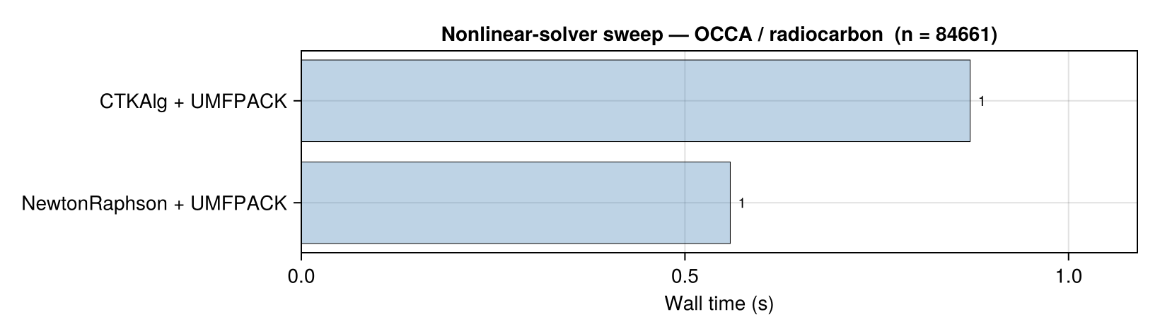
Nonlinear-solver sweep

UMFPACK held fixed; nonlinear algorithm varied.

Tabular timings

Linear-solver sweep — CTKAlg held fixed; linsolve varied

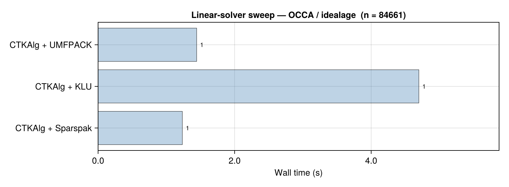
OCCA / idealage (n = 84661)

Algorithm	Scale	Time (s)	Iter	Jrefresh	Lsolves	Max rel drift	τ (yr)	Retcode
CTKAlg + UMFPACK	○	1	1	1	1	4.36e-11	age=8.3e+14	Success
CTKAlg + KLU	○	5	1	1	1	6.92e-11	age=5.4e+14	Success
CTKAlg + Sparspak	○	1	1	1	1	4.18e-11	age=1.2e+15	Success

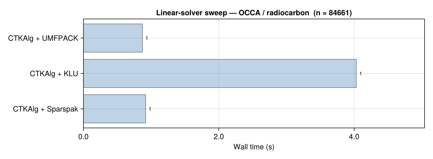
OCCA / radiocarbon (n = 84661)

Algorithm	Scale	Time (s)	Iter	Jrefresh	Lsolves	Max rel drift	τ (yr)	Retcode
CTKAlg + UMFPACK	○	0.87	1	1	1	4.47e-08	R=2.2e+13	Success
CTKAlg + KLU	○	4	1	1	1	7.26e-08	R=1.8e+13	Success
CTKAlg + Sparspak	○	0.92	1	1	1	2.98e-08	R=2.9e+13	Success

OCCA / po4pop (n = 169322)

Algorithm	Scale	Time (s)	Iter	Jrefresh	Lsolves	Max rel drift	τ (yr)	Retcode
CTKAlg + UMFPACK	●	2	9	1	9	2.06e-09	DIP=3.6e+11, POP=1.8e+08	Success
CTKAlg + UMFPACK	○	2	5	1	5	1.09e-05	DIP=6.9e+07, POP=3.4e+04	Success
CTKAlg + KLU	●	5	9	1	9	2.06e-09	DIP=3.6e+11, POP=1.8e+08	Success
CTKAlg + KLU	○	7	5	1	5	1.09e-05	DIP=6.9e+07, POP=3.4e+04	Success
CTKAlg + Sparspak	●	2	9	1	9	2.06e-09	DIP=3.6e+11, POP=1.8e+08	Success
CTKAlg + Sparspak	○	2	5	1	5	1.09e-05	DIP=6.9e+07, POP=3.4e+04	Success

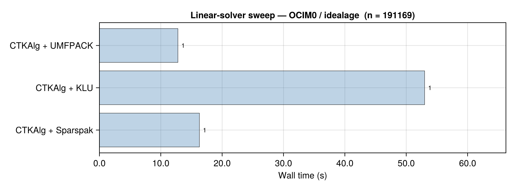
OCIM0 / idealage (n = 191169)

Algorithm	Scale	Time (s)	Iter	Jrefresh	Lsolves	Max rel drift	τ (yr)	Retcode
CTKAlg + UMFPACK	○	13	1	1	1	6.34e-10	age=1.3e+14	Success
CTKAlg + KLU	○	53	1	1	1	7.96e-10	age=8.4e+13	Success
CTKAlg + Sparspak	○	16	1	1	1	4.12e-10	age=1.9e+14	Success

OCIM0 / radiocarbon (n = 191169)

Algorithm	Scale	Time (s)	Iter	Jrefresh	Lsolves	Max rel drift	τ (yr)	Retcode
CTKAlg + UMFPACK	○	4	1	1	1	4.30e-09	R=8.7e+13	Success
CTKAlg + KLU	○	57	1	1	1	1.09e-08	R=5.6e+13	Success
CTKAlg + Sparspak	○	7	1	1	1	3.62e-09	R=1.3e+14	Success

OCIM0 / po4pop (n = 382338)

Algorithm	Scale	Time (s)	Iter	Jrefresh	Lsolves	Max rel drift	τ (yr)	Retcode
CTKAlg + UMFPACK	●	7	3	1	3	5.73e-09	DIP=3.7e+10, POP=2.9e+07	Success
CTKAlg + UMFPACK	○	6	3	1	3	5.73e-09	DIP=3.7e+10, POP=2.9e+07	Success
CTKAlg + KLU	●	55	3	1	3	5.73e-09	DIP=3.7e+10, POP=2.9e+07	Success
CTKAlg + KLU	○	66	3	1	3	5.73e-09	DIP=3.7e+10, POP=2.9e+07	Success
CTKAlg + Sparspak	●	19	3	1	3	5.73e-09	DIP=3.7e+10, POP=2.9e+07	Success
CTKAlg + Sparspak	○	19	3	1	3	5.73e-09	DIP=3.7e+10, POP=2.9e+07	Success

Nonlinear-solver sweep — UMFPACK held fixed; nonlinear algorithm varied

OCCA / idealage (n = 84661)

Algorithm	Scale	Time (s)	Iter	Jrefresh	Lsolves	Max rel drift	τ (yr)	Retcode
CTKAlg + UMFPACK	○	1	1	1	1	4.36e-11	age=8.3e+14	Success
NewtonRaphson + UMFPACK	○	1	1	1	1	4.36e-11	age=8.3e+14	Success

OCCA / radiocarbon (n = 84661)

Algorithm	Scale	Time (s)	Iter	Jrefresh	Lsolves	Max rel drift	τ (yr)	Retcode
CTKAlg + UMFPACK	○	0.87	1	1	1	4.47e-08	R=2.2e+13	Success
NewtonRaphson + UMFPACK	○	0.56	1	1	1	4.47e-08	R=2.2e+13	Success

OCCA / po4pop (n = 169322)

Algorithm	Scale	Time (s)	Iter	Jrefresh	Lsolves	Max rel drift	τ (yr)	Retcode
CTKAlg + UMFPACK	●	2	9	1	9	2.06e-09	DIP=3.6e+11, POP=1.8e+08	Success
CTKAlg + UMFPACK	○	2	5	1	5	1.09e-05	DIP=6.9e+07, POP=3.4e+04	Success
NewtonRaphson + UMFPACK	●	3	3	3	3	1.81e-10	DIP=3.8e+12, POP=1.9e+09	Success
NewtonRaphson + UMFPACK	○	3	3	3	3	1.81e-10	DIP=3.8e+12, POP=1.9e+09	Success

OCIM0 / idealage (n = 191169)

Algorithm	Scale	Time (s)	Iter	Jrefresh	Lsolves	Max rel drift	τ (yr)	Retcode
CTKAlg + UMFPACK	○	13	1	1	1	6.34e-10	age=1.3e+14	Success
NewtonRaphson + UMFPACK	○	6	1	1	1	6.34e-10	age=1.3e+14	Success

OCIM0 / radiocarbon (n = 191169)

Algorithm	Scale	Time (s)	Iter	Jrefresh	Lsolves	Max rel drift	τ (yr)	Retcode
CTKAlg + UMFPACK	○	4	1	1	1	4.30e-09	R=8.7e+13	Success
NewtonRaphson + UMFPACK	○	4	1	1	1	4.30e-09	R=8.7e+13	Success

OCIM0 / po4pop (n = 382338)

Algorithm	Scale	Time (s)	Iter	Jrefresh	Lsolves	Max rel drift	τ (yr)	Retcode
CTKAlg + UMFPACK	●	7	3	1	3	5.73e-09	DIP=3.7e+10, POP=2.9e+07	Success
CTKAlg + UMFPACK	○	6	3	1	3	5.73e-09	DIP=3.7e+10, POP=2.9e+07	Success
NewtonRaphson + UMFPACK	●	42	3	3	3	9.15e-14	DIP=6.9e+14, POP=4.1e+13	Success
NewtonRaphson + UMFPACK	○	18	2	2	2	1.02e-08	DIP=2.5e+10, POP=2e+07	Success

Legend: ● = scaled (nondimensionalize applied); ○ = unscaled (raw original problem).

Last updated: 2026-05-29T15:43:33.792, commit 6ae4b5ab4eca01e64b5d3440a96c6ac27b4f4d35

Future work

Conditional on what the benchmark above shows:

• If the scaled-vs-unscaled comparison shows scaling materially helps in practice, promote benchmark/dimensional_scaling.jl to a supported src/ API with docstring + export, and add a matching how-to walking users through nondimensionalize.

• A "speed vs problem size" log-log scaling plot, which would require the harness to sweep tiers/grid resolutions in a single run (not currently supported).

• A CTKAlg-specific linear-solve counter, wrapping linear_cache, if the iteration / Jacobian-refresh counts alone do not tell the perf story clearly.