Ideal age
The tracer equation for the ideal age is
where the sink term on the right clamps the age to
AIBECS can interpret tracer equations as long as you arrange them under the generic form:
where
In this tutorial, we will simulate the ideal age by
defining functions for
T(p)andG(x,p),defining the parameters
p,generating the state function
F(x,p)and solving the associated steady-state problem,and finally making a plot of our simulated ideal age.
We start by telling Julia that we want to use the AIBECS package and the OCIM2 circulation (the Ocean Circulation Inverse Model[1]).
using AIBECS
using JLD2 # required by `OCIM2.load`
grd, TOCIM2 = OCIM2.load()
(, sparse([1, 2, 10384, 10442, 10443, 20825, 20883, 1, 2, 3 … 200160, 197886, 199766, 199777, 199778, 199779, 199790, 200156, 200159, 200160], [1, 1, 1, 1, 1, 1, 1, 2, 2, 2 … 200159, 200160, 200160, 200160, 200160, 200160, 200160, 200160, 200160, 200160], [0.00019778421518954799, 2.3427916742722093e-9, -1.9599474163829085e-7, -0.00019161212648881556, 4.8096149072091506e-9, -1.830592653460076e-9, 5.007679174162751e-9, -5.025164843241415e-8, 0.00018753126417941492, 4.264266869682882e-8 … -2.196560075226544e-8, 1.0819937104262028e-10, 6.709812718407374e-9, -1.263521554746615e-9, -3.3927920410468295e-9, 7.593163378667893e-9, -7.410175543096161e-9, -3.441057669604186e-8, -2.0030251520181335e-8, 5.2794476107904204e-8], 200160, 200160))Note
If it's your first time, Julia will ask you to download the OCIM2, in which case you should accept (i.e., type y and "return"). Once downloaded, AIBECS will remember where it downloaded the file and it will only load it from your laptop.
grd is an OceanGrid object containing information about the 3D grid of the OCIM2 circulation and TOCIM2 is the transport matrix representing advection and diffusion.
The local sources and sinks for the age take the form
function G(x, p)
    @unpack τ, z₀ = p
    return @. 1 - x / τ * (z ≤ z₀)
end
G (generic function with 1 method)as per the tracer equation. The @unpack line unpacks the parameters τ and z₀. The return line returns the net sources and sinks. (The @. "macro" tells Julia that the operations apply to every element.)
We can define the vector z of depths with depthvec.
z = depthvec(grd)200160-element Vector{Float64}:
18.0675569520817
18.0675569520817
18.0675569520817
18.0675569520817
18.0675569520817
18.0675569520817
18.0675569520817
18.0675569520817
18.0675569520817
18.0675569520817
⋮
5433.2531421838175
5433.2531421838175
5433.2531421838175
5433.2531421838175
5433.2531421838175
5433.2531421838175
5433.2531421838175
5433.2531421838175
5433.2531421838175Now we must construct a type for p the parameters. This type must contain our parameters τ and z₀.
struct IdealAgeParameters{U} <: AbstractParameters{U}
    τ::U
    z₀::U
end
The type is now ready for us to generate an instance of the parameter p. Let's use τ = 1.0 (s) and z₀ the minimum depth of the model.
p = IdealAgeParameters(1.0, z[1])Main.IdealAgeParameters{Float64}
τ = 1.0
z₀ = 18.0675569520817We now use the AIBECS to generate the state function
F = AIBECSFunction(TOCIM2, G)SciMLBase.ODEFunction{false, SciMLBase.AutoSpecialize, AIBECS.var"#f#71"{Tuple{AIBECS.var"#56#57"{SparseMatrixCSC{Float64, Int64}}}, Vector{Int64}, AIBECS.var"#G#68"{Tuple{typeof(Main.G)}, AIBECS.var"#tracers#66"{Int64, Int64}}, AIBECS.var"#tracer#67"{Int64, Int64}}, LinearAlgebra.UniformScaling{Bool}, Nothing, Nothing, AIBECS.var"#jac#81"{AIBECS.var"#T#76"{Tuple{AIBECS.var"#56#57"{SparseMatrixCSC{Float64, Int64}}}, Int64, Vector{Int64}}, AIBECS.var"#72#73"{Tuple{typeof(Main.G)}, Int64, Int64}}, Nothing, Nothing, Nothing, Nothing, Nothing, Nothing, Nothing, Nothing, Nothing, typeof(SciMLBase.DEFAULT_OBSERVED), Nothing, Nothing, Nothing, Nothing}(AIBECS.var"#f#71"{Tuple{AIBECS.var"#56#57"{SparseMatrixCSC{Float64, Int64}}}, Vector{Int64}, AIBECS.var"#G#68"{Tuple{typeof(Main.G)}, AIBECS.var"#tracers#66"{Int64, Int64}}, AIBECS.var"#tracer#67"{Int64, Int64}}((AIBECS.var"#56#57"{SparseMatrixCSC{Float64, Int64}}(sparse([1, 2, 10384, 10442, 10443, 20825, 20883, 1, 2, 3 … 200160, 197886, 199766, 199777, 199778, 199779, 199790, 200156, 200159, 200160], [1, 1, 1, 1, 1, 1, 1, 2, 2, 2 … 200159, 200160, 200160, 200160, 200160, 200160, 200160, 200160, 200160, 200160], [0.00019778421518954799, 2.3427916742722093e-9, -1.9599474163829085e-7, -0.00019161212648881556, 4.8096149072091506e-9, -1.830592653460076e-9, 5.007679174162751e-9, -5.025164843241415e-8, 0.00018753126417941492, 4.264266869682882e-8 … -2.196560075226544e-8, 1.0819937104262028e-10, 6.709812718407374e-9, -1.263521554746615e-9, -3.3927920410468295e-9, 7.593163378667893e-9, -7.410175543096161e-9, -3.441057669604186e-8, -2.0030251520181335e-8, 5.2794476107904204e-8], 200160, 200160)),), [1], AIBECS.var"#G#68"{Tuple{typeof(Main.G)}, AIBECS.var"#tracers#66"{Int64, Int64}}((Main.G,), AIBECS.var"#tracers#66"{Int64, Int64}(200160, 1)), AIBECS.var"#tracer#67"{Int64, Int64}(200160, 1)), LinearAlgebra.UniformScaling{Bool}(true), nothing, nothing, AIBECS.var"#jac#81"{AIBECS.var"#T#76"{Tuple{AIBECS.var"#56#57"{SparseMatrixCSC{Float64, Int64}}}, Int64, Vector{Int64}}, AIBECS.var"#72#73"{Tuple{typeof(Main.G)}, Int64, Int64}}(AIBECS.var"#T#76"{Tuple{AIBECS.var"#56#57"{SparseMatrixCSC{Float64, Int64}}}, Int64, Vector{Int64}}((AIBECS.var"#56#57"{SparseMatrixCSC{Float64, Int64}}(sparse([1, 2, 10384, 10442, 10443, 20825, 20883, 1, 2, 3 … 200160, 197886, 199766, 199777, 199778, 199779, 199790, 200156, 200159, 200160], [1, 1, 1, 1, 1, 1, 1, 2, 2, 2 … 200159, 200160, 200160, 200160, 200160, 200160, 200160, 200160, 200160, 200160], [0.00019778421518954799, 2.3427916742722093e-9, -1.9599474163829085e-7, -0.00019161212648881556, 4.8096149072091506e-9, -1.830592653460076e-9, 5.007679174162751e-9, -5.025164843241415e-8, 0.00018753126417941492, 4.264266869682882e-8 … -2.196560075226544e-8, 1.0819937104262028e-10, 6.709812718407374e-9, -1.263521554746615e-9, -3.3927920410468295e-9, 7.593163378667893e-9, -7.410175543096161e-9, -3.441057669604186e-8, -2.0030251520181335e-8, 5.2794476107904204e-8], 200160, 200160)),), 1, [1]), AIBECS.var"#72#73"{Tuple{typeof(Main.G)}, Int64, Int64}((Main.G,), 200160, 1)), nothing, nothing, nothing, nothing, nothing, nothing, nothing, nothing, nothing, SciMLBase.DEFAULT_OBSERVED, nothing, nothing, nothing, nothing)Now that F and p are defined, we are going to solve for the steady-state. But first, we must create a SteadyStateProblem object that contains F, p, and an initial guess x_init for the age. (SteadyStateProblem comes from SciMLBase.)
Let's make a vector of 0's for our initial guess.
nb = sum(iswet(grd))  # number of wet boxes
x_init = zeros(nb)    # Start with age = 0 everywhere
200160-element Vector{Float64}:
0.0
0.0
0.0
0.0
0.0
0.0
0.0
0.0
0.0
0.0
⋮
0.0
0.0
0.0
0.0
0.0
0.0
0.0
0.0
0.0Now we can create our SteadyStateProblem instance
prob = SteadyStateProblem(F, x_init, p)SteadyStateProblem with uType Vector{Float64}. In-place: false
u0: 200160-element Vector{Float64}:
0.0
0.0
0.0
0.0
0.0
0.0
0.0
0.0
0.0
0.0
⋮
0.0
0.0
0.0
0.0
0.0
0.0
0.0
0.0
0.0And finally, we can solve this problem, using the AIBECS CTKAlg() algorithm,
age = solve(prob, CTKAlg())retcode: MaxIters
u: 200160-element Vector{Float64}:
804.9793529617997
2704.285467766933
559.462475977662
277.6810176373405
571.2245067452848
406.149152964754
416.8838337741092
645.3785433171205
411.6472087934804
242.71573068291767
⋮
1.2204098653557364e10
1.1820841832109226e10
1.3783960333917126e10
1.3083180539737385e10
1.1999572353055943e10
1.1227617212688961e10
1.3402055608211105e10
1.3322655154055128e10
1.212101221557332e10This should take a few seconds.
To conclude this tutorial, let's have a look at the age using AIBECS' plotting recipes and Plots.jl.
using PlotsWe first convert the age in years (because the default SI unit we used, i.e., seconds, is a bit small relative to global ocean timescales).
age_in_yrs = age * u"s" .|> u"yr"200160-element Vector{Quantity{Float64, 𝐓, Unitful.FreeUnits{(yr,), 𝐓, nothing}}}:
2.550825642513371e-5 yr
8.569363537680092e-5 yr
1.7728296067434214e-5 yr
8.799180471180966e-6 yr
1.8101012331269955e-5 yr
1.28700900247406e-5 yr
1.3210251532883019e-5 yr
2.0450811953923e-5 yr
1.3044312900647716e-5 yr
7.691197387726494e-6 yr
⋮
386.7245498249982 yr
374.579874011624 yr
436.78734548625766 yr
414.5809738299929 yr
380.24350245443065 yr
355.78172017799074 yr
424.68551500149266 yr
422.1694664377242 yr
384.09169948200497 yrAnd we take a horizontal slice at about 2000m.
plothorizontalslice(age_in_yrs, grd, depth = 2000u"m", color = :magma)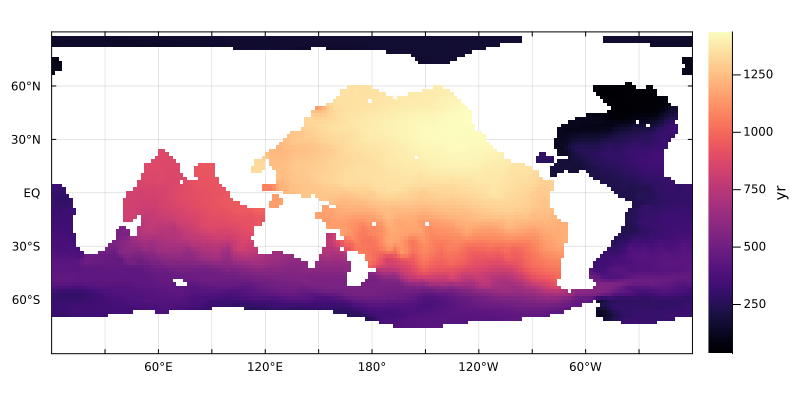
Or look at the horiontal mean
plothorizontalmean(age_in_yrs, grd)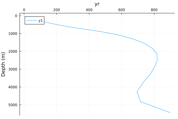
That's it for this tutorial... Good job!
This page was generated using Literate.jl.
DeVries, T., & Holzer, M. (2019). Radiocarbon and helium isotope constraints on deep ocean ventilation and mantle‐³He sources. Journal of Geophysical Research: Oceans, 124, 3036–3057. doi:10.1029/2018JC014716 ↩︎