Groundwater discharge

In this tutorial we will simulate a fictitious radioactive tracer that is injected into the ocean by groundwater discharge. The global groundwater discharge dataset for 40,000 coastal watersheds from Luijendijk et al. (2020) is available from within the AIBECS. Once "born", our ficitious tracer decays with a parameter timescale as it flows through ocean basins.

The 3D tracer equation is:

where   represents the ocean circulation transport. (Tracer transport operators are described in the documentation.) The source of the tracer is , and is the decay rate.

In AIBECS, we must recast this equation in the generic form

We start by telling Julia that we want to use the AIBECS and the OCIM2 transport matrix for the ocean circulation.

using AIBECS
using JLD2                  # required by `OCIM2.load`
using Shapefile, DataFrames # required by `GroundWaters.load`
grd, T_OCIM2 = OCIM2.load()

(, sparse([1, 2, 10384, 10442, 10443, 20825, 20883, 1, 2, 3  …  200160, 197886, 199766, 199777, 199778, 199779, 199790, 200156, 200159, 200160], [1, 1, 1, 1, 1, 1, 1, 2, 2, 2  …  200159, 200160, 200160, 200160, 200160, 200160, 200160, 200160, 200160, 200160], [0.00019778421518954799, 2.3427916742722093e-9, -1.9599474163829085e-7, -0.00019161212648881556, 4.8096149072091506e-9, -1.830592653460076e-9, 5.007679174162751e-9, -5.025164843241415e-8, 0.00018753126417941492, 4.264266869682882e-8  …  -2.196560075226544e-8, 1.0819937104262028e-10, 6.709812718407374e-9, -1.263521554746615e-9, -3.3927920410468295e-9, 7.593163378667893e-9, -7.410175543096161e-9, -3.441057669604186e-8, -2.0030251520181335e-8, 5.2794476107904204e-8], 200160, 200160))

For the radioactive decay, we simply use

function decay(x, p)
    @unpack τ = p
    return x / τ
end

decay (generic function with 1 method)

To build the groundwater sources, we will load the geographic locations and discharge of groundwater (in m³ yr⁻¹) from the Luijendijk et al. (2020)) dataset.

gws = GroundWaters.load()

40409-element Vector{AIBECS.GroundWaters.GroundWaterSource{Quantity{Float64, 𝐋³ 𝐓⁻¹, Unitful.FreeUnits{(m³, yr⁻¹), 𝐋³ 𝐓⁻¹, nothing}}}}:
 AIBECS.GroundWaters.GroundWaterSource{Quantity{Float64, 𝐋³ 𝐓⁻¹, Unitful.FreeUnits{(m³, yr⁻¹), 𝐋³ 𝐓⁻¹, nothing}}}(35.1794887415, 24.2257701314, 47358.8148595 m³ yr⁻¹)
 AIBECS.GroundWaters.GroundWaterSource{Quantity{Float64, 𝐋³ 𝐓⁻¹, Unitful.FreeUnits{(m³, yr⁻¹), 𝐋³ 𝐓⁻¹, nothing}}}(35.3417438136, 23.8746131396, 185142.093516 m³ yr⁻¹)
 AIBECS.GroundWaters.GroundWaterSource{Quantity{Float64, 𝐋³ 𝐓⁻¹, Unitful.FreeUnits{(m³, yr⁻¹), 𝐋³ 𝐓⁻¹, nothing}}}(35.4161096656, 23.6050233764, 171000.541515 m³ yr⁻¹)
 AIBECS.GroundWaters.GroundWaterSource{Quantity{Float64, 𝐋³ 𝐓⁻¹, Unitful.FreeUnits{(m³, yr⁻¹), 𝐋³ 𝐓⁻¹, nothing}}}(35.4266133609, 23.4030494462, 206889.096486 m³ yr⁻¹)
 AIBECS.GroundWaters.GroundWaterSource{Quantity{Float64, 𝐋³ 𝐓⁻¹, Unitful.FreeUnits{(m³, yr⁻¹), 𝐋³ 𝐓⁻¹, nothing}}}(35.7820677063, 22.6137148344, 667545.345579 m³ yr⁻¹)
 AIBECS.GroundWaters.GroundWaterSource{Quantity{Float64, 𝐋³ 𝐓⁻¹, Unitful.FreeUnits{(m³, yr⁻¹), 𝐋³ 𝐓⁻¹, nothing}}}(35.8962644211, 22.6987844211, 72625.201875 m³ yr⁻¹)
 AIBECS.GroundWaters.GroundWaterSource{Quantity{Float64, 𝐋³ 𝐓⁻¹, Unitful.FreeUnits{(m³, yr⁻¹), 𝐋³ 𝐓⁻¹, nothing}}}(35.8614759879, 22.5822032466, 911480.517723 m³ yr⁻¹)
 AIBECS.GroundWaters.GroundWaterSource{Quantity{Float64, 𝐋³ 𝐓⁻¹, Unitful.FreeUnits{(m³, yr⁻¹), 𝐋³ 𝐓⁻¹, nothing}}}(36.6601448123, 21.8794834664, 472586.358228 m³ yr⁻¹)
 AIBECS.GroundWaters.GroundWaterSource{Quantity{Float64, 𝐋³ 𝐓⁻¹, Unitful.FreeUnits{(m³, yr⁻¹), 𝐋³ 𝐓⁻¹, nothing}}}(37.2143679963, 19.334562086, 1.33262583591e6 m³ yr⁻¹)
 AIBECS.GroundWaters.GroundWaterSource{Quantity{Float64, 𝐋³ 𝐓⁻¹, Unitful.FreeUnits{(m³, yr⁻¹), 𝐋³ 𝐓⁻¹, nothing}}}(37.3177380952, 19.3185952381, 28384.2888 m³ yr⁻¹)
 ⋮
 AIBECS.GroundWaters.GroundWaterSource{Quantity{Float64, 𝐋³ 𝐓⁻¹, Unitful.FreeUnits{(m³, yr⁻¹), 𝐋³ 𝐓⁻¹, nothing}}}(144.157841392, 72.2055303019, 11.7123541475 m³ yr⁻¹)
 AIBECS.GroundWaters.GroundWaterSource{Quantity{Float64, 𝐋³ 𝐓⁻¹, Unitful.FreeUnits{(m³, yr⁻¹), 𝐋³ 𝐓⁻¹, nothing}}}(144.236000631, 72.2728170091, 41.4176247705 m³ yr⁻¹)
 AIBECS.GroundWaters.GroundWaterSource{Quantity{Float64, 𝐋³ 𝐓⁻¹, Unitful.FreeUnits{(m³, yr⁻¹), 𝐋³ 𝐓⁻¹, nothing}}}(145.145353536, 71.8562156581, 73.1538069047 m³ yr⁻¹)
 AIBECS.GroundWaters.GroundWaterSource{Quantity{Float64, 𝐋³ 𝐓⁻¹, Unitful.FreeUnits{(m³, yr⁻¹), 𝐋³ 𝐓⁻¹, nothing}}}(128.065238136, 73.2051409179, 105.676353367 m³ yr⁻¹)
 AIBECS.GroundWaters.GroundWaterSource{Quantity{Float64, 𝐋³ 𝐓⁻¹, Unitful.FreeUnits{(m³, yr⁻¹), 𝐋³ 𝐓⁻¹, nothing}}}(143.155736084, 75.5195182604, 93.4943801401 m³ yr⁻¹)
 AIBECS.GroundWaters.GroundWaterSource{Quantity{Float64, 𝐋³ 𝐓⁻¹, Unitful.FreeUnits{(m³, yr⁻¹), 𝐋³ 𝐓⁻¹, nothing}}}(143.243027112, 75.6684283401, 48.7752847061 m³ yr⁻¹)
 AIBECS.GroundWaters.GroundWaterSource{Quantity{Float64, 𝐋³ 𝐓⁻¹, Unitful.FreeUnits{(m³, yr⁻¹), 𝐋³ 𝐓⁻¹, nothing}}}(142.916389905, 75.6972027214, 69.4594679685 m³ yr⁻¹)
 AIBECS.GroundWaters.GroundWaterSource{Quantity{Float64, 𝐋³ 𝐓⁻¹, Unitful.FreeUnits{(m³, yr⁻¹), 𝐋³ 𝐓⁻¹, nothing}}}(128.501004892, 73.1684350529, 87.5895493016 m³ yr⁻¹)
 AIBECS.GroundWaters.GroundWaterSource{Quantity{Float64, 𝐋³ 𝐓⁻¹, Unitful.FreeUnits{(m³, yr⁻¹), 𝐋³ 𝐓⁻¹, nothing}}}(141.832103547, 75.6537345857, 45.9949603817 m³ yr⁻¹)

This is an array of groundwater sources, for which the type GroundWaterSource{T} contains the lat–lon coordinates and discharge in m³ yr⁻¹. For example, the first element is

gws[1]

AIBECS.GroundWaters.GroundWaterSource{Quantity{Float64, 𝐋³ 𝐓⁻¹, Unitful.FreeUnits{(m³, yr⁻¹), 𝐋³ 𝐓⁻¹, nothing}}}(35.1794887415, 24.2257701314, 47358.8148595 m³ yr⁻¹)

We can check the locations with

using Plots
scatter([x.lon for x in gws], [x.lat for x in gws],
        zcolor=log10.(ustrip.([x.VFR for x in gws] / u"m^3/s")),
        colorbartitle="log₁₀(discharge / (1 m³ s⁻¹))",
        clim=(0,10), fmt=:png)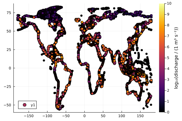

We can regrid these into the OCIM2 grid and return the corresponding vector with

gws_grd = ustrip.(u"m^3/s", regrid(gws, grd))

200160-element Vector{Float64}:
 0.0
 0.0
 0.0
 0.0
 0.0
 0.0
 0.0
 0.0
 0.0
 0.0
 ⋮
 0.0
 0.0
 0.0
 0.0
 0.0
 0.0
 0.0
 0.0
 0.0

(We convert years to seconds for AIBECS)

We can control the global magnitude of the discharge by chosing a concentration of our tracer in groundwater, , in mol m⁻³. For that, we need the volumes of the grid boxes

v = volumevec(grd)

200160-element Vector{Float64}:
 5.693492696598497e11
 6.267656666812283e11
 6.834351352130837e11
 7.392901411788552e11
 7.942641211123751e11
 8.482915614828765e11
 9.013080767686609e11
 9.532504861865775e11
 1.004056888985702e12
 1.053666738215696e12
 ⋮
 2.7437236229729617e13
 2.6923849140323855e13
 2.83653451428806e13
 2.7917925846214992e13
 2.7437236229729617e13
 2.6923849140323855e13
 2.83653451428806e13
 2.7917925846214992e13
 2.7437236229729617e13

because the source is given by the mass (discharge × concentration) divided by the volume of each box:

function s_gw(p)
    @unpack C_gw = p
    return @. gws_grd * C_gw / v
end

s_gw (generic function with 1 method)

We then write the generic function, which is

G_gw(x,p) = s_gw(p) - decay(x,p)

G_gw (generic function with 1 method)

Parameters

We specify some initial values for the parameters and also include units.

import AIBECS: @units, units
import AIBECS: @initial_value, initial_value
@initial_value @units struct GroundWatersParameters{U} <: AbstractParameters{U}
    τ::U    | 20.0 | u"yr"
    C_gw::U |  1.0 | u"mol/m^3"
end

initial_value (generic function with 31 methods)

Finally, thanks to the initial values we provided, we can instantiate the parameter vector succinctly as

p = GroundWatersParameters()

Main.GroundWatersParameters{Float64}
  τ = 20.0 (yr)
  C_gw = 1.0 (mol m⁻³)

We build the state function F,

F = AIBECSFunction(T_OCIM2, G_gw)

SciMLBase.ODEFunction{false, SciMLBase.AutoSpecialize, AIBECS.var"#f#AIBECSFunction##7"{Tuple{AIBECS.var"#AIBECSFunction##0#AIBECSFunction##1"{SparseMatrixCSC{Float64, Int64}}}, Vector{Int64}, AIBECS.var"#G#AIBECSFunction##4"{Tuple{typeof(Main.G_gw)}, AIBECS.var"#tracers#AIBECSFunction##2"{Int64, Int64}}, AIBECS.var"#tracer#AIBECSFunction##3"{Int64, Int64}}, LinearAlgebra.UniformScaling{Bool}, Nothing, Nothing, AIBECS.var"#jac#AIBECSFunction##14"{AIBECS.var"#T#AIBECSFunction##9"{Tuple{AIBECS.var"#AIBECSFunction##0#AIBECSFunction##1"{SparseMatrixCSC{Float64, Int64}}}, Int64, Vector{Int64}}, AIBECS.var"#∇ₓG#AIBECSFunction##8"{Tuple{typeof(Main.G_gw)}, Int64, Int64}}, Nothing, Nothing, Nothing, Nothing, Nothing, Nothing, Nothing, Nothing, Nothing, typeof(SciMLBase.DEFAULT_OBSERVED), Nothing, Nothing, Nothing, Nothing}(AIBECS.var"#f#AIBECSFunction##7"{Tuple{AIBECS.var"#AIBECSFunction##0#AIBECSFunction##1"{SparseMatrixCSC{Float64, Int64}}}, Vector{Int64}, AIBECS.var"#G#AIBECSFunction##4"{Tuple{typeof(Main.G_gw)}, AIBECS.var"#tracers#AIBECSFunction##2"{Int64, Int64}}, AIBECS.var"#tracer#AIBECSFunction##3"{Int64, Int64}}((AIBECS.var"#AIBECSFunction##0#AIBECSFunction##1"{SparseMatrixCSC{Float64, Int64}}(sparse([1, 2, 10384, 10442, 10443, 20825, 20883, 1, 2, 3  …  200160, 197886, 199766, 199777, 199778, 199779, 199790, 200156, 200159, 200160], [1, 1, 1, 1, 1, 1, 1, 2, 2, 2  …  200159, 200160, 200160, 200160, 200160, 200160, 200160, 200160, 200160, 200160], [0.00019778421518954799, 2.3427916742722093e-9, -1.9599474163829085e-7, -0.00019161212648881556, 4.8096149072091506e-9, -1.830592653460076e-9, 5.007679174162751e-9, -5.025164843241415e-8, 0.00018753126417941492, 4.264266869682882e-8  …  -2.196560075226544e-8, 1.0819937104262028e-10, 6.709812718407374e-9, -1.263521554746615e-9, -3.3927920410468295e-9, 7.593163378667893e-9, -7.410175543096161e-9, -3.441057669604186e-8, -2.0030251520181335e-8, 5.2794476107904204e-8], 200160, 200160)),), [1], AIBECS.var"#G#AIBECSFunction##4"{Tuple{typeof(Main.G_gw)}, AIBECS.var"#tracers#AIBECSFunction##2"{Int64, Int64}}((Main.G_gw,), AIBECS.var"#tracers#AIBECSFunction##2"{Int64, Int64}(200160, 1)), AIBECS.var"#tracer#AIBECSFunction##3"{Int64, Int64}(200160, 1)), LinearAlgebra.UniformScaling{Bool}(true), nothing, nothing, AIBECS.var"#jac#AIBECSFunction##14"{AIBECS.var"#T#AIBECSFunction##9"{Tuple{AIBECS.var"#AIBECSFunction##0#AIBECSFunction##1"{SparseMatrixCSC{Float64, Int64}}}, Int64, Vector{Int64}}, AIBECS.var"#∇ₓG#AIBECSFunction##8"{Tuple{typeof(Main.G_gw)}, Int64, Int64}}(AIBECS.var"#T#AIBECSFunction##9"{Tuple{AIBECS.var"#AIBECSFunction##0#AIBECSFunction##1"{SparseMatrixCSC{Float64, Int64}}}, Int64, Vector{Int64}}((AIBECS.var"#AIBECSFunction##0#AIBECSFunction##1"{SparseMatrixCSC{Float64, Int64}}(sparse([1, 2, 10384, 10442, 10443, 20825, 20883, 1, 2, 3  …  200160, 197886, 199766, 199777, 199778, 199779, 199790, 200156, 200159, 200160], [1, 1, 1, 1, 1, 1, 1, 2, 2, 2  …  200159, 200160, 200160, 200160, 200160, 200160, 200160, 200160, 200160, 200160], [0.00019778421518954799, 2.3427916742722093e-9, -1.9599474163829085e-7, -0.00019161212648881556, 4.8096149072091506e-9, -1.830592653460076e-9, 5.007679174162751e-9, -5.025164843241415e-8, 0.00018753126417941492, 4.264266869682882e-8  …  -2.196560075226544e-8, 1.0819937104262028e-10, 6.709812718407374e-9, -1.263521554746615e-9, -3.3927920410468295e-9, 7.593163378667893e-9, -7.410175543096161e-9, -3.441057669604186e-8, -2.0030251520181335e-8, 5.2794476107904204e-8], 200160, 200160)),), 1, [1]), AIBECS.var"#∇ₓG#AIBECSFunction##8"{Tuple{typeof(Main.G_gw)}, Int64, Int64}((Main.G_gw,), 200160, 1)), nothing, nothing, nothing, nothing, nothing, nothing, nothing, nothing, nothing, SciMLBase.DEFAULT_OBSERVED, nothing, nothing, nothing, nothing)

the steady-state problem prob,

nb = sum(iswet(grd))
x = ones(nb) # initial guess
prob = SteadyStateProblem(F, x, p)

SteadyStateProblem with uType Vector{Float64}. In-place: false
u0: 200160-element Vector{Float64}:
 1.0
 1.0
 1.0
 1.0
 1.0
 1.0
 1.0
 1.0
 1.0
 1.0
 ⋮
 1.0
 1.0
 1.0
 1.0
 1.0
 1.0
 1.0
 1.0
 1.0

and solve it

sol = solve(prob, CTKAlg()).u * u"mol/m^3"

200160-element Vector{Quantity{Float64, 𝐍 𝐋⁻³, Unitful.FreeUnits{(m⁻³, mol), 𝐍 𝐋⁻³, nothing}}}:
 -1.1976569114242727e-7 mol m⁻³
 -1.447973438008844e-7 mol m⁻³
 -1.487945316196785e-7 mol m⁻³
 -1.5817358327494297e-7 mol m⁻³
 -1.952022620217977e-7 mol m⁻³
 -2.0677685877026552e-7 mol m⁻³
 -2.244366103876294e-7 mol m⁻³
 -4.112384288419485e-7 mol m⁻³
 -5.599692326820468e-7 mol m⁻³
 -4.4252513643614464e-7 mol m⁻³
  ⋮
  5.356179456772133e-8 mol m⁻³
  9.890403277284479e-8 mol m⁻³
 -1.0615715734082743e-7 mol m⁻³
 -3.777197030624876e-8 mol m⁻³
  7.586448212526303e-8 mol m⁻³
  1.868229167918224e-7 mol m⁻³
 -6.145591682153534e-8 mol m⁻³
 -6.283597352127703e-8 mol m⁻³
  6.068167250824199e-8 mol m⁻³

Let's now run some visualizations using the plot recipes. Taking a horizontal slice of the 3D field at 200m gives

cmap = :viridis
plothorizontalslice(sol, grd, zunit=u"μmol/m^3", depth=200, color=cmap, clim=(0,100))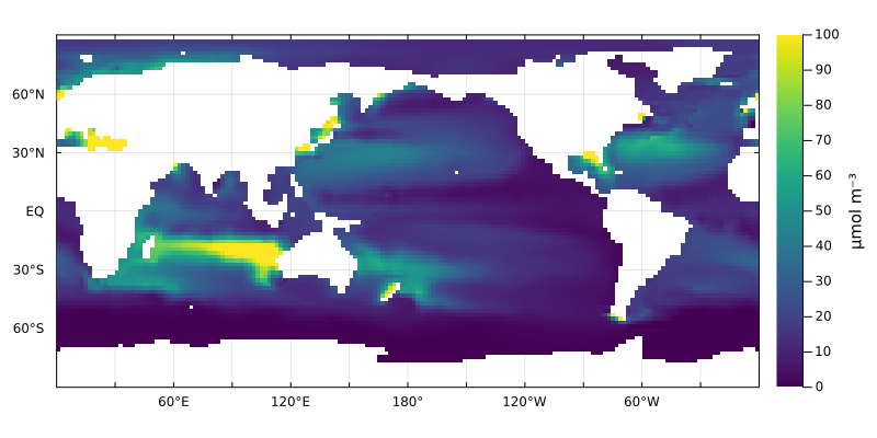

and at 500m:

plothorizontalslice(sol, grd, zunit=u"μmol/m^3", depth=500, color=cmap, clim=(0,25))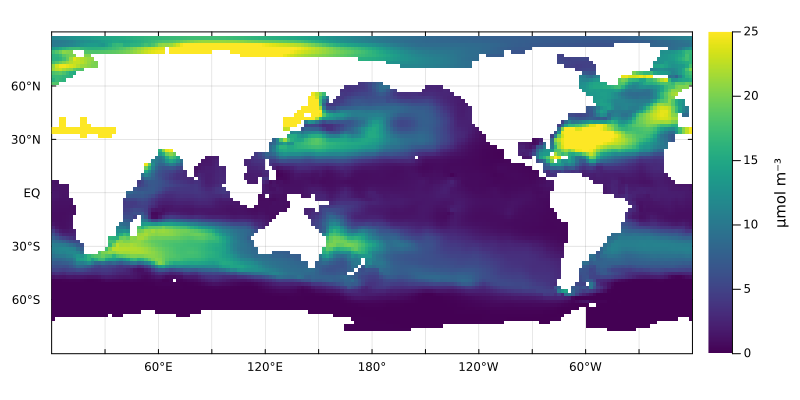

Or we can increase the decay timescale (×10) and decrease the groundwater concentration (÷10) to get a different (more well-mixed) tracer distribution:

p = GroundWatersParameters(τ = 200.0u"yr", C_gw = 0.1u"mol/m^3")
prob = SteadyStateProblem(F, x, p)
sol_τ50 = solve(prob, CTKAlg()).u * u"mol/m^3"
plothorizontalslice(sol_τ50, grd, zunit=u"μmol/m^3", depth=500, color=cmap, clim=(0,25))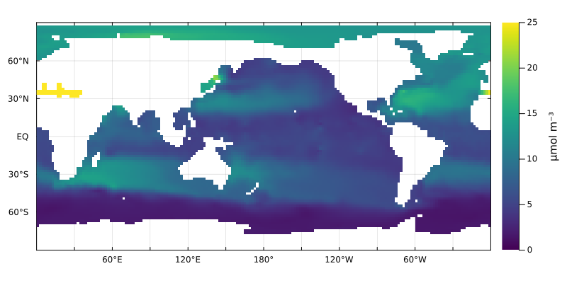

---

This page was generated using Literate.jl.