Tracer transport
Transport operator
To model marine biogeochemical tracers on a global scale we need to be able to account for their movement within the 3D ocean. We do this with tracer transport operators, generically denoted by
In the case of the ocean circulation, i.e., the currents and eddies that transport marine tracers floating around in sea water, the transport operator can be represented by
The
In the case of sinking particles, one can assume that they are only transported downwards with some terminal settling velocity
Discretization
In order to represent a marine tracer on a computer one needs to discretize the 3D ocean into a discrete grid, i.e., a grid with a finite number of boxes. One can go a long way towards understanding what a tracer transport operator is by playing with a simple model with only a few boxes, which is the goal of this piece of documentation.
The simple box model we consider is embedded in a 2×2×2 "shoebox". It has 5 wet boxes and 3 dry boxes, as illustrated below: 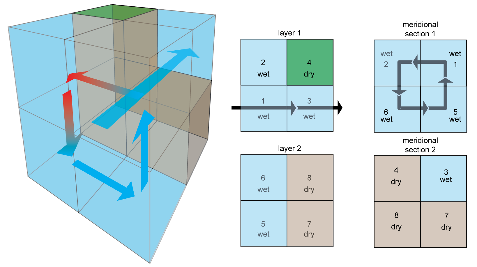
An example of discretized advection,
a meridional overturning circulation flowing in a cycle through boxes 1 → 2 → 6 → 5 → 1 (shown in the meridional section 1 panel)
a zonal current in a reentrant cycling through boxes 1 → 3 → 1 (shown in the layer 1 panel)
Note
This circulation is available as the Primeau_2x2x2 model. You can load it in AIBECS via
grd, T = Primeau_2x2x2.load()Note that this circulation also contains vertical mixing representing deep convection between boxes 2 ↔ 6 (not shown on the image)
Vectorization
In AIBECS, tracers are represented by column vectors. That is, the 3D tracer field, 
The continuous transport operator
Note
A sparse matrix behaves the same way as a regular matrix. The only difference is that in a sparse matrix the majority of the entries are zeros. These zeros are not stored explicitly to save computer memory making it possible to deal with fairly high resolution ocean models.
Mathematically, the discretization and vectorization convert an expression with partial derivatives into a matrix vector product. In summary, for the ocean circulation, we do the following conversion
Ocean circulations in AIBECS
In AIBECS, there are currently a few available circulations that you can directly load with the AIBECS:
TwoBoxModel, the 2-box model of the Sarmiento and Gruber (2006) bookPrimeau_2x2x2, the circulation described in this documentation pageArcher_etal_2000, the 3-box model of Archer et al. (2000) (also used in the Sarmiento and Gruber (2006) book)Haine_and_Hall_2025, the 9-box pedagogical circulation of Haine and Hall (2002), as described in Haine et al. (2025)OCIM0, the unnamed precursor of the OCIM1 (and which should actually be named OCIM0.1)OCIM1OCIM2OCIM2_48L, the higher vertical-resolution variant of OCIM2OCCA
To load any of these, you just need to do
grd, T = Circulation.load()where Circulation is one of the circulations listed above.
If you are adventurous, you can create your own circulations. AIBECS provides some tools for this. (This is how the Primeau_2x2x2 and Archer_etal_2000 circulations were created.)
Sinking particles in AIBECS
There are no loadable transport operators for sinking particles, because there are too many ways to represent sinking particles. However, the AIBECS provides tools to create your own transport operators by providing a scalar or a vector of the downward settling velocities, w. For example, you can create the transport operator for particles sinking at 100 m/d everywhere simply via
T = transportoperator(grd, w=100u"m/d")