Sinking particles

This how-to walks through building transport operators for sinking particles — the second kind of transport in AIBECS, alongside the advection–diffusion of dissolved tracers. It complements the Estimate fluxes how-to, which decomposes an existing circulation by direction.

using AIBECS, Plots
using JLD2 # required by `OCIM2.load`

Loading a grid

We will use OCIM2 throughout.

grd, _ = OCIM2.load()

(, sparse([1, 2, 10384, 10442, 10443, 20825, 20883, 1, 2, 3  …  200160, 197886, 199766, 199777, 199778, 199779, 199790, 200156, 200159, 200160], [1, 1, 1, 1, 1, 1, 1, 2, 2, 2  …  200159, 200160, 200160, 200160, 200160, 200160, 200160, 200160, 200160, 200160], [0.00019778421518954799, 2.3427916742722093e-9, -1.9599474163829085e-7, -0.00019161212648881556, 4.8096149072091506e-9, -1.830592653460076e-9, 5.007679174162751e-9, -5.025164843241415e-8, 0.00018753126417941492, 4.264266869682882e-8  …  -2.196560075226544e-8, 1.0819937104262028e-10, 6.709812718407374e-9, -1.263521554746615e-9, -3.3927920410468295e-9, 7.593163378667893e-9, -7.410175543096161e-9, -3.441057669604186e-8, -2.0030251520181335e-8, 5.2794476107904204e-8], 200160, 200160))

Constant settling velocity

The simplest case: particles fall everywhere at the same speed.

T_const = transportoperator(grd, 100.0)  # 100 m/s in SI units

200160×200160 SparseMatrixCSC{Float64, Int64} with 379438 stored entries:
⎡⠑⢄⠀⠀⠀⠀⠀⠀⠀⠀⠀⠀⠀⠀⠀⠀⠀⠀⠀⠀⠀⠀⠀⠀⠀⠀⠀⠀⠀⠀⠀⠀⠀⠀⠀⠀⠀⠀⠀⠀⎤
⎢⠳⣄⠑⢄⠀⠀⠀⠀⠀⠀⠀⠀⠀⠀⠀⠀⠀⠀⠀⠀⠀⠀⠀⠀⠀⠀⠀⠀⠀⠀⠀⠀⠀⠀⠀⠀⠀⠀⠀⠀⎥
⎢⠀⠈⠳⣄⠑⢄⠀⠀⠀⠀⠀⠀⠀⠀⠀⠀⠀⠀⠀⠀⠀⠀⠀⠀⠀⠀⠀⠀⠀⠀⠀⠀⠀⠀⠀⠀⠀⠀⠀⠀⎥
⎢⠀⠀⠀⠈⠳⣄⠑⢄⠀⠀⠀⠀⠀⠀⠀⠀⠀⠀⠀⠀⠀⠀⠀⠀⠀⠀⠀⠀⠀⠀⠀⠀⠀⠀⠀⠀⠀⠀⠀⠀⎥
⎢⠀⠀⠀⠀⠀⠈⠳⣄⠑⢄⠀⠀⠀⠀⠀⠀⠀⠀⠀⠀⠀⠀⠀⠀⠀⠀⠀⠀⠀⠀⠀⠀⠀⠀⠀⠀⠀⠀⠀⠀⎥
⎢⠀⠀⠀⠀⠀⠀⠀⠈⠳⣄⠑⢄⠀⠀⠀⠀⠀⠀⠀⠀⠀⠀⠀⠀⠀⠀⠀⠀⠀⠀⠀⠀⠀⠀⠀⠀⠀⠀⠀⠀⎥
⎢⠀⠀⠀⠀⠀⠀⠀⠀⠀⠈⠳⣄⠑⢄⠀⠀⠀⠀⠀⠀⠀⠀⠀⠀⠀⠀⠀⠀⠀⠀⠀⠀⠀⠀⠀⠀⠀⠀⠀⠀⎥
⎢⠀⠀⠀⠀⠀⠀⠀⠀⠀⠀⠀⠈⠓⢦⡑⢄⠀⠀⠀⠀⠀⠀⠀⠀⠀⠀⠀⠀⠀⠀⠀⠀⠀⠀⠀⠀⠀⠀⠀⠀⎥
⎢⠀⠀⠀⠀⠀⠀⠀⠀⠀⠀⠀⠀⠀⠀⠙⢦⡑⢄⠀⠀⠀⠀⠀⠀⠀⠀⠀⠀⠀⠀⠀⠀⠀⠀⠀⠀⠀⠀⠀⠀⎥
⎢⠀⠀⠀⠀⠀⠀⠀⠀⠀⠀⠀⠀⠀⠀⠀⠀⠙⢦⡑⢄⠀⠀⠀⠀⠀⠀⠀⠀⠀⠀⠀⠀⠀⠀⠀⠀⠀⠀⠀⠀⎥
⎢⠀⠀⠀⠀⠀⠀⠀⠀⠀⠀⠀⠀⠀⠀⠀⠀⠀⠀⠙⢦⡑⢄⠀⠀⠀⠀⠀⠀⠀⠀⠀⠀⠀⠀⠀⠀⠀⠀⠀⠀⎥
⎢⠀⠀⠀⠀⠀⠀⠀⠀⠀⠀⠀⠀⠀⠀⠀⠀⠀⠀⠀⠀⠙⢦⡑⢄⠀⠀⠀⠀⠀⠀⠀⠀⠀⠀⠀⠀⠀⠀⠀⠀⎥
⎢⠀⠀⠀⠀⠀⠀⠀⠀⠀⠀⠀⠀⠀⠀⠀⠀⠀⠀⠀⠀⠀⠀⠙⢦⡑⢄⠀⠀⠀⠀⠀⠀⠀⠀⠀⠀⠀⠀⠀⠀⎥
⎢⠀⠀⠀⠀⠀⠀⠀⠀⠀⠀⠀⠀⠀⠀⠀⠀⠀⠀⠀⠀⠀⠀⠀⠀⠙⢦⡑⢄⠀⠀⠀⠀⠀⠀⠀⠀⠀⠀⠀⠀⎥
⎢⠀⠀⠀⠀⠀⠀⠀⠀⠀⠀⠀⠀⠀⠀⠀⠀⠀⠀⠀⠀⠀⠀⠀⠀⠀⠀⠙⢦⡑⢄⠀⠀⠀⠀⠀⠀⠀⠀⠀⠀⎥
⎢⠀⠀⠀⠀⠀⠀⠀⠀⠀⠀⠀⠀⠀⠀⠀⠀⠀⠀⠀⠀⠀⠀⠀⠀⠀⠀⠀⠀⠙⢦⡑⢄⠀⠀⠀⠀⠀⠀⠀⠀⎥
⎢⠀⠀⠀⠀⠀⠀⠀⠀⠀⠀⠀⠀⠀⠀⠀⠀⠀⠀⠀⠀⠀⠀⠀⠀⠀⠀⠀⠀⠀⠀⠙⢦⡑⢄⠀⠀⠀⠀⠀⠀⎥
⎢⠀⠀⠀⠀⠀⠀⠀⠀⠀⠀⠀⠀⠀⠀⠀⠀⠀⠀⠀⠀⠀⠀⠀⠀⠀⠀⠀⠀⠀⠀⠀⠀⠙⢦⡑⢄⠀⠀⠀⠀⎥
⎢⠀⠀⠀⠀⠀⠀⠀⠀⠀⠀⠀⠀⠀⠀⠀⠀⠀⠀⠀⠀⠀⠀⠀⠀⠀⠀⠀⠀⠀⠀⠀⠀⠀⠀⠉⠳⣕⢄⠀⠀⎥
⎣⠀⠀⠀⠀⠀⠀⠀⠀⠀⠀⠀⠀⠀⠀⠀⠀⠀⠀⠀⠀⠀⠀⠀⠀⠀⠀⠀⠀⠀⠀⠀⠀⠀⠀⠀⠀⠈⠓⢷⣄⎦

T_const is a sparse matrix; multiplying by a tracer vector returns its flux divergence due to sinking.

Depth-dependent settling velocity

Pass a function w(z) to make the settling speed grow with depth — a common parameterisation. Here w(z) = 2z + 1, with no remineralisation at the seafloor (fsedremin = 0.0 means all particles arriving at the seafloor are considered remineralised in place rather than reflected back).

T_var = transportoperator(grd, z -> 2z + 1; fsedremin = 0.0)

200160×200160 SparseMatrixCSC{Float64, Int64} with 389879 stored entries:
⎡⠑⢄⠀⠀⠀⠀⠀⠀⠀⠀⠀⠀⠀⠀⠀⠀⠀⠀⠀⠀⠀⠀⠀⠀⠀⠀⠀⠀⠀⠀⠀⠀⠀⠀⠀⠀⠀⠀⠀⠀⎤
⎢⠳⣄⠑⢄⠀⠀⠀⠀⠀⠀⠀⠀⠀⠀⠀⠀⠀⠀⠀⠀⠀⠀⠀⠀⠀⠀⠀⠀⠀⠀⠀⠀⠀⠀⠀⠀⠀⠀⠀⠀⎥
⎢⠀⠈⠳⣄⠑⢄⠀⠀⠀⠀⠀⠀⠀⠀⠀⠀⠀⠀⠀⠀⠀⠀⠀⠀⠀⠀⠀⠀⠀⠀⠀⠀⠀⠀⠀⠀⠀⠀⠀⠀⎥
⎢⠀⠀⠀⠈⠳⣄⠑⢄⠀⠀⠀⠀⠀⠀⠀⠀⠀⠀⠀⠀⠀⠀⠀⠀⠀⠀⠀⠀⠀⠀⠀⠀⠀⠀⠀⠀⠀⠀⠀⠀⎥
⎢⠀⠀⠀⠀⠀⠈⠳⣄⠑⢄⠀⠀⠀⠀⠀⠀⠀⠀⠀⠀⠀⠀⠀⠀⠀⠀⠀⠀⠀⠀⠀⠀⠀⠀⠀⠀⠀⠀⠀⠀⎥
⎢⠀⠀⠀⠀⠀⠀⠀⠈⠳⣄⠑⢄⠀⠀⠀⠀⠀⠀⠀⠀⠀⠀⠀⠀⠀⠀⠀⠀⠀⠀⠀⠀⠀⠀⠀⠀⠀⠀⠀⠀⎥
⎢⠀⠀⠀⠀⠀⠀⠀⠀⠀⠈⠳⣄⠑⢄⠀⠀⠀⠀⠀⠀⠀⠀⠀⠀⠀⠀⠀⠀⠀⠀⠀⠀⠀⠀⠀⠀⠀⠀⠀⠀⎥
⎢⠀⠀⠀⠀⠀⠀⠀⠀⠀⠀⠀⠈⠓⢦⡑⢄⠀⠀⠀⠀⠀⠀⠀⠀⠀⠀⠀⠀⠀⠀⠀⠀⠀⠀⠀⠀⠀⠀⠀⠀⎥
⎢⠀⠀⠀⠀⠀⠀⠀⠀⠀⠀⠀⠀⠀⠀⠙⢦⡑⢄⠀⠀⠀⠀⠀⠀⠀⠀⠀⠀⠀⠀⠀⠀⠀⠀⠀⠀⠀⠀⠀⠀⎥
⎢⠀⠀⠀⠀⠀⠀⠀⠀⠀⠀⠀⠀⠀⠀⠀⠀⠙⢦⡑⢄⠀⠀⠀⠀⠀⠀⠀⠀⠀⠀⠀⠀⠀⠀⠀⠀⠀⠀⠀⠀⎥
⎢⠀⠀⠀⠀⠀⠀⠀⠀⠀⠀⠀⠀⠀⠀⠀⠀⠀⠀⠙⢦⡑⢄⠀⠀⠀⠀⠀⠀⠀⠀⠀⠀⠀⠀⠀⠀⠀⠀⠀⠀⎥
⎢⠀⠀⠀⠀⠀⠀⠀⠀⠀⠀⠀⠀⠀⠀⠀⠀⠀⠀⠀⠀⠙⢦⡑⢄⠀⠀⠀⠀⠀⠀⠀⠀⠀⠀⠀⠀⠀⠀⠀⠀⎥
⎢⠀⠀⠀⠀⠀⠀⠀⠀⠀⠀⠀⠀⠀⠀⠀⠀⠀⠀⠀⠀⠀⠀⠙⢦⡑⢄⠀⠀⠀⠀⠀⠀⠀⠀⠀⠀⠀⠀⠀⠀⎥
⎢⠀⠀⠀⠀⠀⠀⠀⠀⠀⠀⠀⠀⠀⠀⠀⠀⠀⠀⠀⠀⠀⠀⠀⠀⠙⢦⡑⢄⠀⠀⠀⠀⠀⠀⠀⠀⠀⠀⠀⠀⎥
⎢⠀⠀⠀⠀⠀⠀⠀⠀⠀⠀⠀⠀⠀⠀⠀⠀⠀⠀⠀⠀⠀⠀⠀⠀⠀⠀⠙⢦⡑⢄⠀⠀⠀⠀⠀⠀⠀⠀⠀⠀⎥
⎢⠀⠀⠀⠀⠀⠀⠀⠀⠀⠀⠀⠀⠀⠀⠀⠀⠀⠀⠀⠀⠀⠀⠀⠀⠀⠀⠀⠀⠙⢦⡑⢄⠀⠀⠀⠀⠀⠀⠀⠀⎥
⎢⠀⠀⠀⠀⠀⠀⠀⠀⠀⠀⠀⠀⠀⠀⠀⠀⠀⠀⠀⠀⠀⠀⠀⠀⠀⠀⠀⠀⠀⠀⠙⢦⡑⢄⠀⠀⠀⠀⠀⠀⎥
⎢⠀⠀⠀⠀⠀⠀⠀⠀⠀⠀⠀⠀⠀⠀⠀⠀⠀⠀⠀⠀⠀⠀⠀⠀⠀⠀⠀⠀⠀⠀⠀⠀⠙⢦⡑⢄⠀⠀⠀⠀⎥
⎢⠀⠀⠀⠀⠀⠀⠀⠀⠀⠀⠀⠀⠀⠀⠀⠀⠀⠀⠀⠀⠀⠀⠀⠀⠀⠀⠀⠀⠀⠀⠀⠀⠀⠀⠉⠳⣕⢄⠀⠀⎥
⎣⠀⠀⠀⠀⠀⠀⠀⠀⠀⠀⠀⠀⠀⠀⠀⠀⠀⠀⠀⠀⠀⠀⠀⠀⠀⠀⠀⠀⠀⠀⠀⠀⠀⠀⠀⠀⠈⠓⢷⣄⎦

Inspecting the building blocks

Internally transportoperator is PFDO = DIVO * FATO — a flux-at-top operator (FATO) composed with a vertical divergence (DIVO):

DIVOp = DIVO(grd)
Iabove = buildIabove(grd)
F = FATO(fill(100.0, count(iswet(grd))), Iabove)
P = PFDO(fill(100.0, count(iswet(grd))), DIVOp, Iabove)

200160×200160 SparseMatrixCSC{Float64, Int64} with 379438 stored entries:
⎡⠑⢄⠀⠀⠀⠀⠀⠀⠀⠀⠀⠀⠀⠀⠀⠀⠀⠀⠀⠀⠀⠀⠀⠀⠀⠀⠀⠀⠀⠀⠀⠀⠀⠀⠀⠀⠀⠀⠀⠀⎤
⎢⠳⣄⠑⢄⠀⠀⠀⠀⠀⠀⠀⠀⠀⠀⠀⠀⠀⠀⠀⠀⠀⠀⠀⠀⠀⠀⠀⠀⠀⠀⠀⠀⠀⠀⠀⠀⠀⠀⠀⠀⎥
⎢⠀⠈⠳⣄⠑⢄⠀⠀⠀⠀⠀⠀⠀⠀⠀⠀⠀⠀⠀⠀⠀⠀⠀⠀⠀⠀⠀⠀⠀⠀⠀⠀⠀⠀⠀⠀⠀⠀⠀⠀⎥
⎢⠀⠀⠀⠈⠳⣄⠑⢄⠀⠀⠀⠀⠀⠀⠀⠀⠀⠀⠀⠀⠀⠀⠀⠀⠀⠀⠀⠀⠀⠀⠀⠀⠀⠀⠀⠀⠀⠀⠀⠀⎥
⎢⠀⠀⠀⠀⠀⠈⠳⣄⠑⢄⠀⠀⠀⠀⠀⠀⠀⠀⠀⠀⠀⠀⠀⠀⠀⠀⠀⠀⠀⠀⠀⠀⠀⠀⠀⠀⠀⠀⠀⠀⎥
⎢⠀⠀⠀⠀⠀⠀⠀⠈⠳⣄⠑⢄⠀⠀⠀⠀⠀⠀⠀⠀⠀⠀⠀⠀⠀⠀⠀⠀⠀⠀⠀⠀⠀⠀⠀⠀⠀⠀⠀⠀⎥
⎢⠀⠀⠀⠀⠀⠀⠀⠀⠀⠈⠳⣄⠑⢄⠀⠀⠀⠀⠀⠀⠀⠀⠀⠀⠀⠀⠀⠀⠀⠀⠀⠀⠀⠀⠀⠀⠀⠀⠀⠀⎥
⎢⠀⠀⠀⠀⠀⠀⠀⠀⠀⠀⠀⠈⠓⢦⡑⢄⠀⠀⠀⠀⠀⠀⠀⠀⠀⠀⠀⠀⠀⠀⠀⠀⠀⠀⠀⠀⠀⠀⠀⠀⎥
⎢⠀⠀⠀⠀⠀⠀⠀⠀⠀⠀⠀⠀⠀⠀⠙⢦⡑⢄⠀⠀⠀⠀⠀⠀⠀⠀⠀⠀⠀⠀⠀⠀⠀⠀⠀⠀⠀⠀⠀⠀⎥
⎢⠀⠀⠀⠀⠀⠀⠀⠀⠀⠀⠀⠀⠀⠀⠀⠀⠙⢦⡑⢄⠀⠀⠀⠀⠀⠀⠀⠀⠀⠀⠀⠀⠀⠀⠀⠀⠀⠀⠀⠀⎥
⎢⠀⠀⠀⠀⠀⠀⠀⠀⠀⠀⠀⠀⠀⠀⠀⠀⠀⠀⠙⢦⡑⢄⠀⠀⠀⠀⠀⠀⠀⠀⠀⠀⠀⠀⠀⠀⠀⠀⠀⠀⎥
⎢⠀⠀⠀⠀⠀⠀⠀⠀⠀⠀⠀⠀⠀⠀⠀⠀⠀⠀⠀⠀⠙⢦⡑⢄⠀⠀⠀⠀⠀⠀⠀⠀⠀⠀⠀⠀⠀⠀⠀⠀⎥
⎢⠀⠀⠀⠀⠀⠀⠀⠀⠀⠀⠀⠀⠀⠀⠀⠀⠀⠀⠀⠀⠀⠀⠙⢦⡑⢄⠀⠀⠀⠀⠀⠀⠀⠀⠀⠀⠀⠀⠀⠀⎥
⎢⠀⠀⠀⠀⠀⠀⠀⠀⠀⠀⠀⠀⠀⠀⠀⠀⠀⠀⠀⠀⠀⠀⠀⠀⠙⢦⡑⢄⠀⠀⠀⠀⠀⠀⠀⠀⠀⠀⠀⠀⎥
⎢⠀⠀⠀⠀⠀⠀⠀⠀⠀⠀⠀⠀⠀⠀⠀⠀⠀⠀⠀⠀⠀⠀⠀⠀⠀⠀⠙⢦⡑⢄⠀⠀⠀⠀⠀⠀⠀⠀⠀⠀⎥
⎢⠀⠀⠀⠀⠀⠀⠀⠀⠀⠀⠀⠀⠀⠀⠀⠀⠀⠀⠀⠀⠀⠀⠀⠀⠀⠀⠀⠀⠙⢦⡑⢄⠀⠀⠀⠀⠀⠀⠀⠀⎥
⎢⠀⠀⠀⠀⠀⠀⠀⠀⠀⠀⠀⠀⠀⠀⠀⠀⠀⠀⠀⠀⠀⠀⠀⠀⠀⠀⠀⠀⠀⠀⠙⢦⡑⢄⠀⠀⠀⠀⠀⠀⎥
⎢⠀⠀⠀⠀⠀⠀⠀⠀⠀⠀⠀⠀⠀⠀⠀⠀⠀⠀⠀⠀⠀⠀⠀⠀⠀⠀⠀⠀⠀⠀⠀⠀⠙⢦⡑⢄⠀⠀⠀⠀⎥
⎢⠀⠀⠀⠀⠀⠀⠀⠀⠀⠀⠀⠀⠀⠀⠀⠀⠀⠀⠀⠀⠀⠀⠀⠀⠀⠀⠀⠀⠀⠀⠀⠀⠀⠀⠉⠳⣕⢄⠀⠀⎥
⎣⠀⠀⠀⠀⠀⠀⠀⠀⠀⠀⠀⠀⠀⠀⠀⠀⠀⠀⠀⠀⠀⠀⠀⠀⠀⠀⠀⠀⠀⠀⠀⠀⠀⠀⠀⠀⠈⠓⢷⣄⎦

P is T_const with the same content; exposing the pieces is useful when you want to compose the flux differently (e.g. attach a remineralisation profile, or feed FATO with a non-uniform w_top).

Plotting the flux divergence

Apply the operator to a uniform tracer field of 1 mol m⁻³ and plot a meridional slice of the resulting flux divergence:

x = ones(count(iswet(grd)))
divϕ = -T_var * x * u"mol/m^3/s" .|> u"μmol/m^3/d"
plotmeridionalslice(divϕ, grd, lon = 330)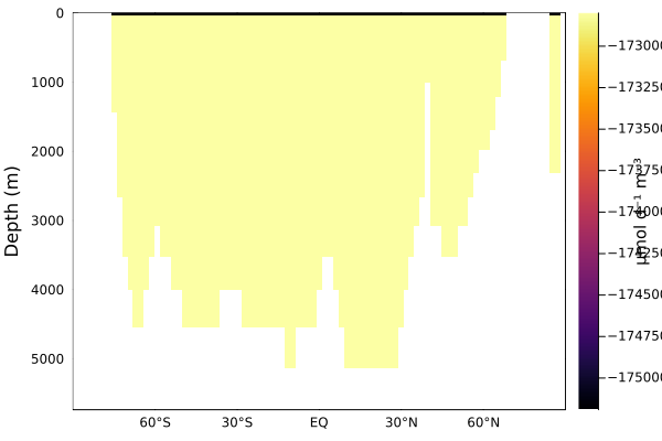

A negative divergence means the box is losing tracer to sinking out of the bottom; a positive divergence means it is gaining from particles settling in from above.

---

This page was generated using Literate.jl.