Radiocarbon

In this tutorial, we will simulate the radiocarbon age using the AIBECS by

defining the transport T(p) and the sources and sinks G(x,p),
defining the parameters p,
generating the state function F(x,p) and solving the associated steady-state problem,
and finally making a plot of our simulated radiocarbon age.

Note

Although this tutorial is self-contained, it is slightly more complicated than the first tutorial for simulating the ideal age. (So do not hesitate to start with the idealage tutorial if you wish.)

The tracer equation for radiocarbon is

where the first term on the right of the equal sign represents the air–sea gas exchange with a piston velocity over a depth and the second term represents the radioactive decay of radiocarbon with timescale .

Note

We need not specify the value of the atmospheric radiocarbon concentration because it is not important for determining the age of a water parcel — only the relative concentration matters.

We start by selecting the circulation for Radiocarbon.

(And this time, we are using the OCCA matrix by Forget (2010) ^[1].)

julia

using AIBECS
using JLD2 # required by `OCCA.load`
grd, T_OCCA = OCCA.load()

(, sparse([1, 2, 9551, 9606, 1, 2, 3, 57, 9552, 9607  …  79928, 84632, 84659, 84660, 84661, 79891, 79929, 84633, 84660, 84661], [1, 1, 1, 1, 2, 2, 2, 2, 2, 2  …  84660, 84660, 84660, 84660, 84660, 84661, 84661, 84661, 84661, 84661], [2.2826279842870655e-7, 1.8030621712982388e-10, -2.202759122121374e-7, -1.669794081839543e-8, -8.32821319857397e-8, 3.6454996849707203e-7, -2.4345873581518986e-8, 2.346272528650749e-8, -3.294980961099172e-7, 6.798120022902578e-9  …  -2.337773104642457e-8, -1.0853897038905248e-8, -2.4801404742669764e-8, 7.658935255067088e-8, -2.49410804832536e-8, -2.2788300189327118e-9, -3.386139290468414e-8, -2.0539768803799346e-8, -1.8193948479846445e-8, 5.864674518359535e-8], 84661, 84661))

The local sources and sinks are simply given by

julia

function G(R, p)
    @unpack λ, h, Ratm, τ = p
    return @. λ / h * (Ratm - R) * (z ≤ h) - R / τ
end

G (generic function with 1 method)

We can define z via

julia

z = depthvec(grd)

84661-element Vector{Float64}:
   25.0
   25.0
   25.0
   25.0
   25.0
   25.0
   25.0
   25.0
   25.0
   25.0
    ⋮
 5062.25
 5062.25
 5062.25
 5062.25
 5062.25
 5062.25
 5062.25
 5062.25
 5062.25

In this tutorial we will specify some units for the parameters. Such features must be imported to be used

julia

import AIBECS: @units, units

We define the parameters using the dedicated API from the AIBECS, including keyword arguments and units this time

julia

@units struct RadiocarbonParameters{U} <: AbstractParameters{U}
    λ::U    | u"m/yr"
    h::U    | u"m"
    τ::U    | u"yr"
    Ratm::U | u"M"
end

units (generic function with 53 methods)

For the air–sea gas exchange, we use a constant piston velocity of 50m / 10years. And for the radioactive decay we use a timescale of 5730/log(2) years.

julia

p = RadiocarbonParameters(
    λ = 50u"m" / 10u"yr",
    h = grd.δdepth[1],
    τ = 5730u"yr" / log(2),
    Ratm = 42.0u"nM"
)

Main.RadiocarbonParameters{Float64}
  λ = 5.0 (m yr⁻¹)
  h = 50.0 (m)
  τ = 8266.64258429376 (yr)
  Ratm = 4.2000000000000006e-8 (M)

Note

The parameters are converted to SI units when unpacked. When you specify units for your parameters, you must either supply their values in that unit.

We build the state function F and the corresponding steady-state problem (and solve it) via

julia

F = AIBECSFunction(T_OCCA, G)
x = zeros(length(z)) # an initial guess
prob = SteadyStateProblem(F, x, p)
R = solve(prob, CTKAlg()).u

84661-element Vector{Float64}:
 3.782989042400264e-5
 3.777181712272232e-5
 3.660371729335564e-5
 3.707310908733552e-5
 3.716239375219126e-5
 3.7168497048614304e-5
 3.709453566001736e-5
 3.7159561038925754e-5
 3.723606252569647e-5
 3.7349967402672724e-5
 ⋮
 3.635099586594514e-5
 3.634755896919857e-5
 3.6339096931777565e-5
 3.6347484352324805e-5
 3.63826810104347e-5
 3.6421920073910325e-5
 3.647280866120177e-5
 3.6488010171142744e-5
 3.650169024828974e-5

This should take a few seconds on a laptop. Once the radiocarbon concentration is computed, we can convert it into the corresponding age in years, via

julia

@unpack τ, Ratm = p
C14age = @. log(Ratm / R) * τ * u"s" |> u"yr"

84661-element Vector{Quantity{Float64, 𝐓, Unitful.FreeUnits{(yr,), 𝐓, nothing}}}:
  864.4434447899139 yr
  877.1434574053698 yr
 1136.827180697325 yr
 1031.4929288324006 yr
 1011.6079751302298 yr
 1010.2504299781357 yr
 1026.7165651310008 yr
 1012.2381261585998 yr
  995.2368392305344 yr
  969.9878310854215 yr
    ⋮
 1194.1001375754036 yr
 1194.881765135638 yr
 1196.8065376635063 yr
 1194.8987355093514 yr
 1186.897702814917 yr
 1177.9868554324005 yr
 1166.4447909128373 yr
 1163.0000529492802 yr
 1159.9013058938976 yr

and plot it at 700 m using the horizontalslice Plots recipe

julia

using Plots
plothorizontalslice(C14age, grd, depth = 700u"m", color = :viridis)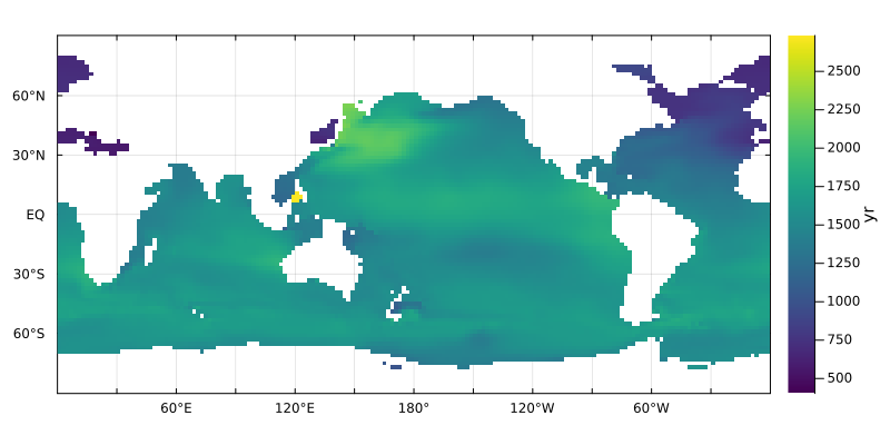

look at a zonal average using the zonalaverage plot recipe

julia

plotzonalaverage(C14age, grd; color = :viridis)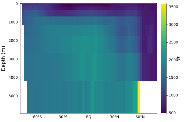

or look at a meridional slice through the Atlantic at 30°W using the meridionalslice plot recipe

julia

plotmeridionalslice(C14age, grd, lon = -30, color = :viridis)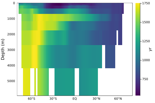

This page was generated using Literate.jl.

Forget, G., 2010: Mapping Ocean Observations in a Dynamical Framework: A 2004–06 Ocean Atlas. J. Phys. Oceanogr., 40, 1201–1221, doi:10.1175/2009JPO4043.1) ↩︎

Radiocarbon ​

Radiocarbon